[ML] Bayes Classifier

Posted May 24, 2026

By Jina Kim 28 min read

Classification Problem

Feature vector $\mathbf{x}$와 qualitative response $\mathbf{y}$가 주어졌을 때, $\mathbf{y}$의 값을 예측하는 함수 $f(\mathbf{x}) \in C$를 만드는 것이 목표.
보통은 어떤 확률 분포 $p(\mathbf{x}, \mathbf{y})$에서 i.i.d.로 샘플된 $n$개의 training data $(\mathbf{x}^{(i)}, \mathbf{y}^{(i)})$가 있다고 가정.
즉, classification은 $\mathbf{x}$에서 $\mathbf{y}$로 가는 function approximation 문제.

Bayes Classifier

Risk와 Bayes Classifier의 정의

classifier $f: \mathbf{x} \to \mathbf{y}$에 대해, Risk $R(f)$는

\[R(f) = \mathbb{E}_{p(\mathbf{x}, \mathbf{y})}[\mathcal{L}(\mathbf{y}, f(\mathbf{x}))] = \sum_{\mathbf{x}} \sum_{\mathbf{y}} p(\mathbf{x}, \mathbf{y}) \mathcal{L}(\mathbf{y}, f(\mathbf{x}))\]

Risk는 expected loss

Bayes Classifier $f^*$는 이 risk를 최소화하는 classifier.

\[f^* = \arg\min_f \mathbb{E}_{p(\mathbf{x}, \mathbf{y})}[\mathcal{L}(\mathbf{y}, f(\mathbf{x}))]\]

개별 $x$에 대해서는

\[f^*(x) = \arg\min_{\hat{\mathbf{y}}} \sum_{\mathbf{y}} p(\mathbf{y}|\mathbf{x} = x) \mathcal{L}(\mathbf{y}, \hat{\mathbf{y}})\]

Binary 세팅에서의 유도

binary classification $\mathbf{y} \in {+1, -1}$ 케이스에서 풀어 쓰면,

\[\begin{aligned} f^*(x) &= \arg\min_{\hat{\mathbf{y}}} \sum_{\mathbf{y}} p(\mathbf{y}\|\mathbf{x} = x) \mathcal{L}(\mathbf{y}, \hat{\mathbf{y}}) \\ &= \arg\min_{\hat{\mathbf{y}}} p(\mathbf{y}=1|\mathbf{x}=x)\mathcal{L}(1, \hat{\mathbf{y}}) + p(\mathbf{y}=-1|\mathbf{x}=x)\mathcal{L}(-1, \hat{\mathbf{y}}) \end{aligned}\]

y가 1이면 loss $\mathcal{L}(1, \hat{\mathbf{y}})$ 가 0
y가 -1이면 loss $\mathcal{L}(-1, \hat{\mathbf{y}})$ 가 0
posterior가 큰 쪽의 loss를 zero-out 시키는 게 이득임
$p(\mathbf{y}=1|x) > p(\mathbf{y}=-1|x)$ → $\hat{y} = +1$
$p(\mathbf{y}=1|x) < p(\mathbf{y}=-1|x)$ → $\hat{y} = -1$

이걸 sign과 log를 써서 한 줄로 정리하면,

\[\begin{aligned} f^*(x) &= \arg\min_{\hat{\mathbf{y}}} p(\mathbf{y}=1|\mathbf{x}=x)\mathcal{L}(1, \hat{\mathbf{y}}) + p(\mathbf{y}=-1|\mathbf{x}=x)\mathcal{L}(-1, \hat{\mathbf{y}}) \\ &= \text{sign}\left(\log \frac{p(\mathbf{y}=1|\mathbf{x}=x)}{p(\mathbf{y}=-1|\mathbf{x}=x)}\right) \end{aligned}\]

$\log \frac{p(\mathbf{y}=1|\mathbf{x}=x)}{p(\mathbf{y}=-1|\mathbf{x}=x)}$ 가 양수가 나오면 sign 값이 +1
$\log \frac{p(\mathbf{y}=1|\mathbf{x}=x)}{p(\mathbf{y}=-1|\mathbf{x}=x)}$ 가 음수가 나오면 sign 값이 -1
- 부호만 갖다 쓰고 싶을 때 사용
$p(\mathbf{y}=1|x) > p(\mathbf{y}=-1|x)$ 일 때 log 안의 값이 1보다 커져 → log값 양수 → sign +1
$p(\mathbf{y}=1|x) < p(\mathbf{y}=-1|x)$ 일 때 log 안의 값이 1보다 작아져 → log값 음수 → sign -1

Bayes’ Rule 적용

우리가 알고 싶은 건 posterior $p(\mathbf{y}|\mathbf{x})$인데, 이걸 직접 모델링하기 힘드니까 Bayes’ Rule로 뒤집어 봄.

\[p(\mathbf{y}\|\mathbf{x}) = \frac{p(\mathbf{x}\|\mathbf{y}) p(\mathbf{y})}{p(\mathbf{x})}\]

Prior $p(\mathbf{y})$: $\mathbf{x}$를 보기 전 라벨의 확률
Likelihood $p(\mathbf{x}|\mathbf{y})$: 클래스 $\mathbf{y}$에서 $\mathbf{x}$가 관측될 확률
Posterior $p(\mathbf{y}|\mathbf{x})$: $\mathbf{x}$를 본 후 라벨의 확률

따라서,

\[f^*(x) = \text{sign}\left(\log \frac{p(\mathbf{x}=x\|\mathbf{y}=1)p(\mathbf{y}=1)}{p(\mathbf{x}=x|\mathbf{y}=-1)p(\mathbf{y}=-1)}\right)\]

$p(\mathbf{x})$는 분자/분모 비율에서 cancel out
prior와 likelihood는 데이터로부터 추정하기 훨씬 쉬움

Discriminant Analysis

두 가지 Classification 전략

문제는 우리가 $p(\mathbf{x}, \mathbf{y})$를 모른다는 것. training data로 추정해야 함.

Generative classifier
MLE로 $p(\mathbf{x}|\mathbf{y})$와 $p(\mathbf{y})$를 추정 → Bayes’ Rule로 합침.
- ex.) Bayes classifier, Discriminant Analysis
Discriminative classifier
$p(\mathbf{y}|\mathbf{x})$를 Bayes’ Rule 없이 직접 추정.
- ex.) Logistic regression

Gaussian 가정

$f^*(x)$를 근사하기 위해 $p(\mathbf{x}|\mathbf{y})$가 Gaussian $\mathcal{N}(\mu_y, \Sigma_y)$이라고 가정함.

\[\begin{aligned} f^*(x) &= \text{sign}\left(\log \frac{p(\mathbf{x}=x\|\mathbf{y}=1)p(\mathbf{y}=1)}{p(\mathbf{x}=x\|\mathbf{y}=-1)p(\mathbf{y}=-1)}\right) \\ &= \text{sign}\left(\log \frac{\mathcal{N}(\mu_1, \sigma_1) \cdot \alpha}{\mathcal{N}(\mu_{-1}, \sigma_{-1}) \cdot (1-\alpha)}\right) \end{aligned}\]

$\hat{\alpha}$ : $p(\mathbf{y}=1)$의 추정값
- $p(\mathbf{y}=-1) = 1 - \hat{\alpha}$
$\hat{\mu}_1$, $\hat{\mu}_{-1}$: 각 클래스 데이터의 평균
$\hat{\Sigma}_1$, $\hat{\Sigma}_{-1}$: 각 클래스 데이터의 공분산 행렬

신만이 아는 두 개의 Gaussian 분포가 있고, 샘플 $\mathbf{x}$는 그 중 하나에서 나왔다고 믿음
분포는 모르지만 샘플이 있으니, 샘플로부터 $(\mu, \Sigma)$를 추정
그 다음 새로운 $\mathbf{x}’$에 대해 각 분포에서 나왔을 확률을 비교해서 분류
Prior는 개별 샘플과 무관하게 각 클래스 확률을 보정해주는 역할.

1D Case 풀어 쓰기

$\mathbf{x}$가 scalar라고 두면 Gaussian

\[\mathcal{N}(\mu, \sigma^2) = \frac{1}{\sqrt{2\pi\sigma^2}} e^{-\frac{(\mathbf{x}-\mu)^2}{2\sigma^2}}\]

을 $f^*(x)$에 그대로 대입:

\[f^*(x) = \mathrm{sign}\left(\log \frac{\mathcal{N}(\mu_1, \sigma_1) \cdot \alpha}{\mathcal{N}(\mu_{-1}, \sigma_{-1}) \cdot (1-\alpha)}\right)\] \[= \mathrm{sign}\left(\log \frac{\dfrac{1}{\sqrt{2\pi\sigma_1^2}} e^{-\frac{(\mathbf{x}-\mu_1)^2}{2\sigma_1^2}} \cdot \alpha}{\dfrac{1}{\sqrt{2\pi\sigma_{-1}^2}} e^{-\frac{(\mathbf{x}-\mu_{-1})^2}{2\sigma_{-1}^2}} \cdot (1-\alpha)}\right)\]

log 안의 분수를 풀면 (log의 곱은 합, 나눗셈은 차, 지수는 앞으로),

\[= \mathrm{sign}\left(-\log \frac{\sqrt{2\pi\sigma_1^2}}{\sqrt{2\pi\sigma_{-1}^2}} - \frac{(\mathbf{x}-\mu_1)^2}{2\sigma_1^2} + \frac{(\mathbf{x}-\mu_{-1})^2}{2\sigma_{-1}^2} + \log \frac{\alpha}{1-\alpha}\right)\]

$\sqrt{2\pi}$가 분자분모에서 약분되어 사라지고, 남은 $\sqrt{\sigma_1^2} / \sqrt{\sigma_{-1}^2}$의 log는 $\frac{1}{2}\log(\sigma_1^2/\sigma_{-1}^2)$로 정리됨:

\[f^*(x) = \mathrm{sign}\left(-\frac{1}{2}\log \frac{\sigma_1^2}{\sigma_{-1}^2} - \frac{(\mathbf{x}-\mu_1)^2}{2\sigma_1^2} + \frac{(\mathbf{x}-\mu_{-1})^2}{2\sigma_{-1}^2} + \log \frac{\alpha}{1-\alpha}\right)\]

여기서 $\mu_1, \mu_{-1}, \sigma_1^2, \sigma_{-1}^2$를 데이터로부터 추정해야 함.

MLE로 파라미터 추정

Log-likelihood를 세움:

\[\ell(\mu_1, \mu_{-1}, \sigma_1, \sigma_{-1}) = \log \prod_{i=1}^{n} p(\mathbf{x}_i | \mathbf{y}_i)\]

클래스별로 곱을 쪼개면,

\[= \log \left[\prod_{i: \mathbf{y}_i=1} p(\mathbf{x}_i|\mathbf{y}_i) \prod_{j: \mathbf{y}_j=-1} p(\mathbf{x}_j|\mathbf{y}_j)\right]\] \[= \sum_{i:\mathbf{y}_i=1} \log p(\mathbf{x}_i|\mathbf{y}_i) + \sum_{j:\mathbf{y}_j=-1} \log p(\mathbf{x}_j|\mathbf{y}_j)\]

각 항은 Gaussian이니까,

\[= \sum_{i:\mathbf{y}_i=1} \log \frac{1}{\sigma_1\sqrt{2\pi}} e^{-\frac{(\mathbf{x}_i-\mu_1)^2}{2\sigma_1^2}} + \sum_{i:\mathbf{y}_i=-1} \log \frac{1}{\sigma_{-1}\sqrt{2\pi}} e^{-\frac{(\mathbf{x}_i-\mu_{-1})^2}{2\sigma_{-1}^2}}\]

log 안의 지수를 밖으로 빼면,

\[\ell = \sum_{i:\mathbf{y}_i=1} \log \frac{1}{\sigma_1\sqrt{2\pi}} - \frac{1}{2\sigma_1^2}\sum_{i:\mathbf{y}_i=1}(\mathbf{x}_i - \mu_1)^2 + \sum_{i:\mathbf{y}_i=-1} \log \frac{1}{\sigma_{-1}\sqrt{2\pi}} - \frac{1}{2\sigma_{-1}^2}\sum_{i:\mathbf{y}_i=-1}(\mathbf{x}_i - \mu_{-1})^2\]

$\mu_1$에 대해 편미분:

\[\frac{\partial \ell}{\partial \mu_1} = -\frac{1}{\sigma_1^2}\sum_{i:\mathbf{y}_i=1}(\mathbf{x}_i - \mu_1) = 0\] \[\implies \sum_{i:\mathbf{y}_i=1} \mathbf{x}_i = \sum_{i:\mathbf{y}_i=1} \mu_1 \implies \hat{\mu}_1 = \frac{1}{n_1}\sum_{i:\mathbf{y}_i=1} \mathbf{x}_i\]

class 1에 해당하는 데이터에 대한 평균
$n_1$은 클래스 +1의 training data 개수

$\sigma_1$에 대해 편미분:

\[\frac{\partial \ell}{\partial \sigma_1} = -\frac{n_1}{\sigma_1} - \frac{1}{2}\cdot(-2)\sigma_1^{-3}\sum_{i:\mathbf{y}_i=1}(\mathbf{x}_i-\mu_1)^2 = 0\] \[\implies \frac{n_1}{\sigma_1} = \frac{1}{\sigma_1^3}\sum_{i:\mathbf{y}_i=1}(\mathbf{x}_i-\mu_1)^2 \implies \hat{\sigma}*1^2 = \frac{1}{n_1}\sum_{i:\mathbf{y}_i=1}(\mathbf{x}_i - \mu_1)^2\]

$\dfrac{\partial \ell}{\partial \mu_{-1}}$, $\dfrac{\partial \ell}{\partial \sigma_{-1}}$도 똑같이 풀면 대칭적으로:

\[\hat{\mu}_{-1} = \frac{1}{n_{-1}}\sum_{i:\mathbf{y}_i=-1} \mathbf{x}_i, \qquad \hat{\sigma}_{-1}^2 = \frac{1}{n_{-1}}\sum_{i:\mathbf{y}_i=-1}(\mathbf{x}_i - \mu_{-1})^2\]

$\hat{\mu}_{{1,-1}}$ : 클래스별 평균
$\hat{\sigma}_{{1,-1}}^2$ : 클래스별 표준편차

LDA (Linear Discriminant Analysis)

위 일반화된 수식을 간략화 하기 위해 “각각의 클래스가 평균은 다르지만 분산은 같은 것이다”라는

추가 가정: $\hat{\sigma}_1^2 = \hat{\sigma}_{-1}^2 = \hat{\sigma}^2$

1D case 식부터 다시 출발:

$\sigma_1^2 = \sigma_{-1}^2 = \sigma^2$를 대입하면 첫 번째 log 항은 $\log(\sigma^2/\sigma^2) = \log 1 = 0$이라 사라짐:

\[= \mathrm{sign}\left(\cancel{-\frac{1}{2}\log \frac{\sigma^2}{\sigma^2}} - \frac{(\mathbf{x}-\mu_1)^2}{2\sigma^2} + \frac{(\mathbf{x}-\mu_{-1})^2}{2\sigma^2} + \log \frac{\alpha}{1-\alpha}\right)\]

두 분수를 묶으면,

\[= \mathrm{sign}\left(-\frac{1}{2\sigma^2}\left((\mathbf{x}-\mu_1)^2 - (\mathbf{x}-\mu_{-1})^2\right) + \log \frac{\alpha}{1-\alpha}\right)\]

제곱을 전개:

\[= \mathrm{sign}\left(-\frac{1}{2\sigma^2}(\cancel{\mathbf{x}^2} - 2\mu_1 \mathbf{x} + \mu_1^2 - \cancel{\mathbf{x}^2} + 2\mu_{-1}\mathbf{x} - \mu_{-1}^2) + \log \frac{\alpha}{1-\alpha}\right)\]

$\mathbf{x}^2$ 항이 서로 상쇄되는 게 핵심. 정리하면,

\[\boxed{f^*(x) = \mathrm{sign}\left(\frac{1}{\sigma^2}(\mu_1 - \mu_{-1})\mathbf{x} - \frac{1}{2\sigma^2}(\mu_1^2 - \mu_{-1}^2) + \log \frac{\alpha}{1-\alpha}\right)}\]

$\mathbf{x}$에 대해 1차 (linear) 형태가 됨. 이게 LDA의 핵심.

QDA (Quadratic Discriminant Analysis)

$\hat{\sigma}_1^2 = \hat{\sigma}_{-1}^2$ 가정을 안 하면 $\mathbf{x}^2$ 항이 약분 안 되고 살아남음. 즉,

가 그대로 second-order polynomial in $\mathbf{x}$. 더 표현력 있지만 추정할 파라미터가 많아짐.

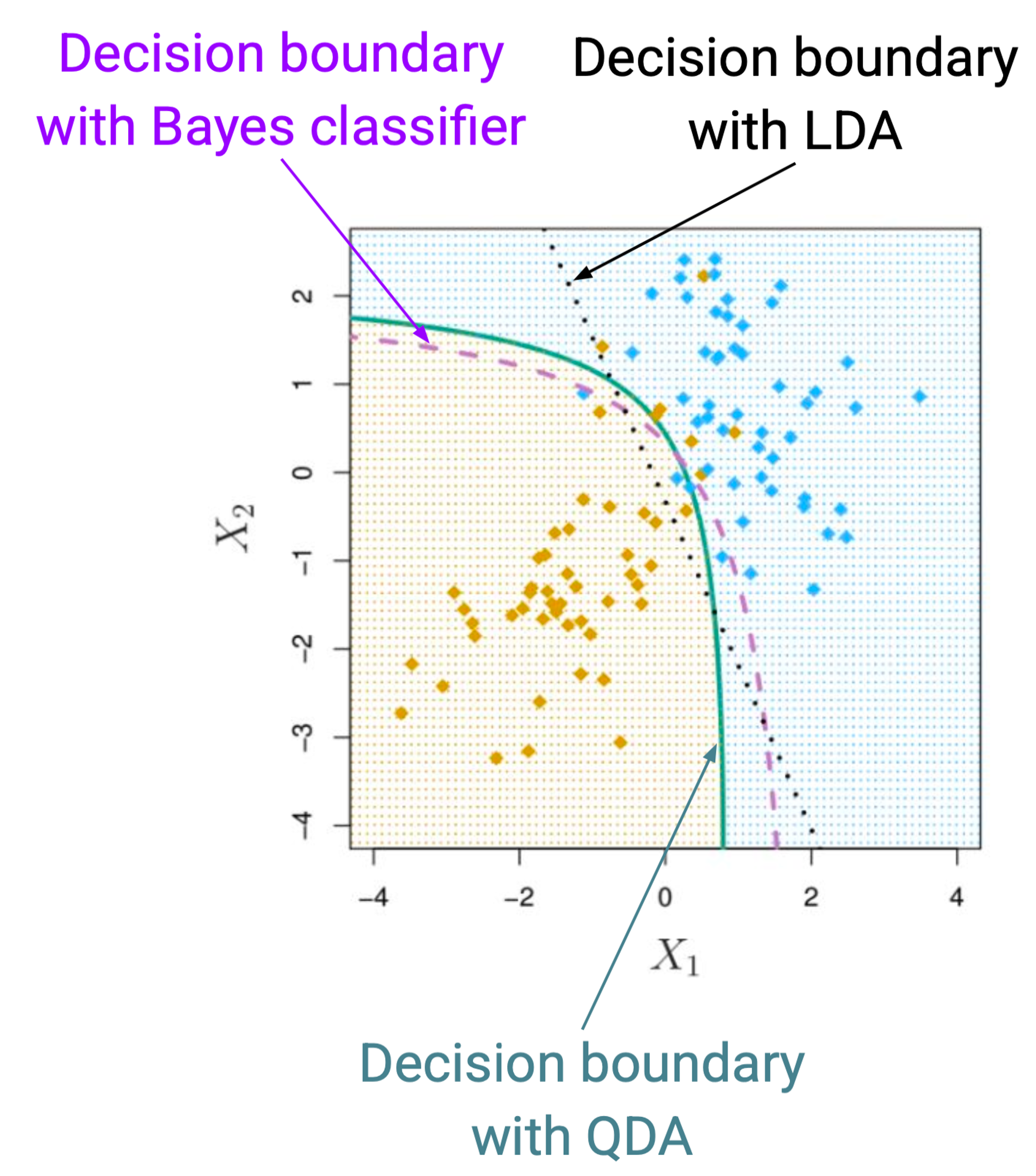
보라색 boundary가 실제 데이터셋의 boundary
LDA, QDA로 학습을 시켰을 때, 데이터셋을 보고 두 클래스를 어떻게 분류하는지
QDA가 더 비슷하긴 함

다차원 Discriminant Analysis

$d$-차원 Gaussian:

\[\mathcal{N}(\mu_y, \Sigma_y) = (2\pi)^{-\frac{d}{2}} |\Sigma_y|^{-\frac{1}{2}} e^{-\frac{1}{2}(\mathbf{x}-\mu_y)^\top \Sigma_y^{-1}(\mathbf{x}-\mu_y)}\]

$d$: input dimensionality
$\mathbf{x}, \mu_y \in \mathbb{R}^d$: $d$-차원 input/mean vector
$\Sigma_y \in \mathbb{R}^{d \times d}$: covariance matrix

다차원 LDA discriminant function:

\[\delta_k(\mathbf{x}) = \mathbf{x}^\top \Sigma^{-1} \mu_k - \frac{1}{2}\mu_k^\top \Sigma^{-1} \mu_k + \log \alpha_k\]

1D case와 비교:

\[\delta_k(\mathbf{x}) = \frac{\mu_k}{\sigma^2}\mathbf{x} - \frac{\mu_k^2}{2\sigma^2} + \log \alpha_k\]

형태가 자연스럽게 일반화됨. 곱셈 → 행렬 곱.
$\sigma^2 \to \Sigma$
$\mu \to \mu_k$

cf) 공분산 행렬은, $\mathrm{Cov}(\mathbf{X}) = \begin{bmatrix} \mathrm{Cov}(X, X) & \mathrm{Cov}(Y, X) \ \mathrm{Cov}(X, Y) & \mathrm{Cov}(Y, Y) \end{bmatrix} = \begin{bmatrix} \dfrac{\sum (x_i-\bar{X})(x_i-\bar{X})}{N} & \dfrac{\sum (x_i-\bar{X})(y_i-\bar{Y})}{N} \ \dfrac{\sum (x_i-\bar{X})(y_i-\bar{Y})}{N} & \dfrac{\sum (y_i-\bar{Y})(y_i-\bar{Y})}{N} \end{bmatrix}$

2D 예시; 일반적으로 $d \times d$.

3+ Class로 확장

LDA의 binary 식을 다시 가져옴:

\[f^*(x) = \mathrm{sign}\left(\frac{1}{\sigma^2}(\mu_1 - \mu_{-1})\mathbf{x} - \frac{1}{2\sigma^2}(\mu_1^2 - \mu_{-1}^2) + \log \frac{\alpha}{1-\alpha}\right)\]

이걸 각 클래스에 해당하는 항으로 쪼개면 (log 비율도 분리),

\[= \mathrm{sign}\left(\left(\frac{\mu_1}{\sigma^2}\mathbf{x} - \frac{\mu_1^2}{2\sigma^2} + \log \alpha\right) - \left(\frac{\mu_{-1}}{\sigma^2}\mathbf{x} - \frac{\mu_{-1}^2}{2\sigma^2} + \log (1-\alpha)\right)\right)\]

부호로 케이스 분류:

\[= \begin{cases} +1 & \text{if } \dfrac{\mu_1}{\sigma^2}\mathbf{x} - \dfrac{\mu_1^2}{2\sigma^2} + \log \alpha \geq \dfrac{\mu_{-1}}{\sigma^2}\mathbf{x} - \dfrac{\mu_{-1}^2}{2\sigma^2} + \log(1-\alpha) \\ -1 & \text{if } \dfrac{\mu_1}{\sigma^2}\mathbf{x} - \dfrac{\mu_1^2}{2\sigma^2} + \log \alpha < \dfrac{\mu_{-1}}{\sigma^2}\mathbf{x} - \dfrac{\mu_{-1}^2}{2\sigma^2} + \log(1-\alpha) \end{cases}\]

prior 부분을 각각 $\alpha = \alpha_1$로 놓고, $1 - \alpha = \alpha_{-1}$로 놓으면 두 클래스가 같은 scoring form을 가짐:

\[= \begin{cases} +1 & \text{if } \dfrac{\mu_1}{\sigma^2}\mathbf{x} - \dfrac{\mu_1^2}{2\sigma^2} + \log \alpha_1 \geq \dfrac{\mu_{-1}}{\sigma^2}\mathbf{x} - \dfrac{\mu_{-1}^2}{2\sigma^2} + \log \alpha_{-1} \\ -1 & \text{otherwise} \end{cases}\]

즉, 클래스 $k$에 대한 discriminant score:

\[\boxed{\delta_k(\mathbf{x}) = \frac{\mu_k}{\sigma^2}\mathbf{x} - \frac{\mu_k^2}{2\sigma^2} + \log \alpha_k}\]

3개 이상 클래스에서는 각 클래스에 대해 $\delta_k(\mathbf{x})$를 계산하고 가장 높은 score를 갖는 클래스로 분류하면 됨.

Softmax (Score $\rightarrow$ 확률)

$\hat{\delta}_k(\mathbf{x})$로부터 estimated class probability를 얻고 싶으면 softmax 적용:

\[\hat{\mathbb{P}}(Y = k | X = x) = \frac{e^{\hat{\delta}*k(x)}}{\sum_{\ell=1}^{K} e^{\hat{\delta}_\ell(x)}}\]

이렇게 하면 가장 큰 $\hat{\delta}_k(\mathbf{x})$를 갖는 클래스로 분류하면서 동시에 confidence도 얻음.

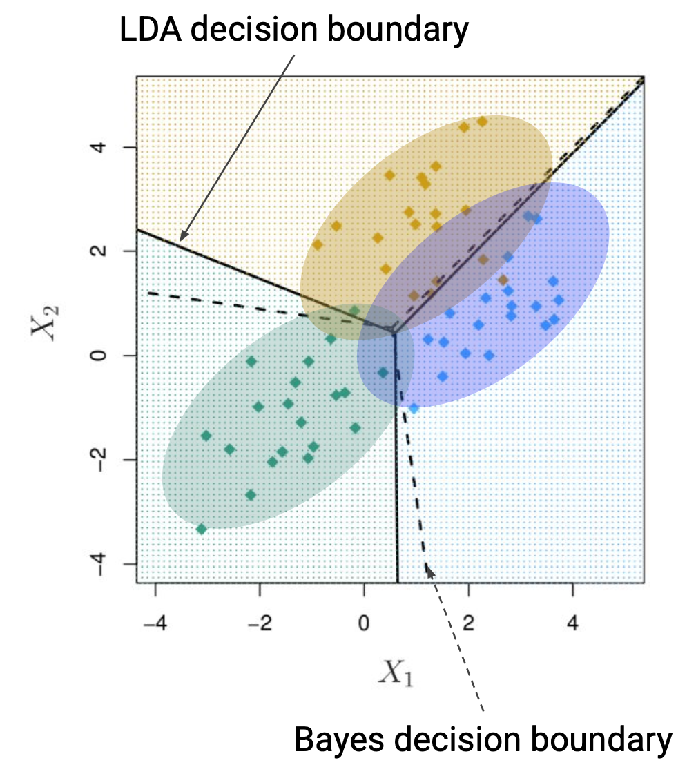
3개 이상의 클래스가 있을 때

클래스 별로 평균과 분산 값 구해서 각각의 정규분포 생성
- 다른 클래스 데이터 신경 쓰지 말고, 각각의 클래스 데이터 모아서 계산
이 케이스에서
- $\alpha_1 = \alpha_2 = \alpha_3$ 이라서 3개 클래스에 대해 따로 가중치 없음
- $\sum = \sum_1 = \sum_2 = \sum_3$ 이라서 gaussian distribution 모양이 똑같다
Bayes decision boundary : 이 데이터를 생성할 때 사용했던 진실된 확률분포
LDA decision boundary : 3개의 확률값을 구해서 가장 높게 나타나는 영역을 기준으로 나눠놓은 것

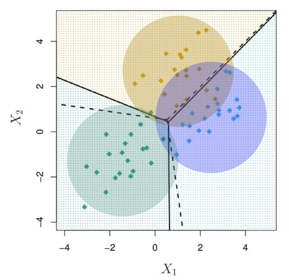
분산 모델링을 해서 지금 타원형인데, $\sum = \sum_1 = \sum_2 = \sum_3 = \mathbf{I}$로 두면 원이 됨.
분산은 데이터로부터 찾는 게 아니라 같은 값을 갖는다고 해버리니까 클래스마다 모양이 똑같음

Discriminant Analysis는 왜 쓰는가?

클래스가 well-separated일 때, logistic regression의 파라미터 추정이 굉장히 불안정함.
- 중간에 샘플이 별로 없어서 decision boundary 정하기 어려워
- LDA는 이 문제 없음.
$n$이 작고 각 클래스의 예측 변수 분포가 approximately normal이면, LDA가 logistic regression보다 더 stable.
- LDA의 가정이 잘 맞아떨어지는 케이스
2개 이상 클래스에서 많이 사용함
- 데이터의 low-dimensional view도 제공해줌.

LDA vs. Logistic Regression

공통점

2-class 문제에서는 LDA와 logistic regression이 같은 form을 가짐:

\[\log\left(\frac{p_1(x)}{1 - p_1(x)}\right) = \log\left(\frac{p_1(x)}{p_2(x)}\right) = c_0 + c_1 x_1 + \cdots + c_p x_p\]

각각 풀어 쓰면,

Logistic regression:

\[\log\left(\frac{p(X;\boldsymbol{\beta})}{1 - p(X;\boldsymbol{\beta})}\right) = \beta_0 + \beta_1 X_1 + \cdots + \beta_p X_p\]

LDA:

\[f^*(x) = \mathrm{sign}\left(\log \frac{\mathcal{N}(\mu_1, \sigma_1) \cdot \alpha}{\mathcal{N}(\mu_{-1}, \sigma_{-1}) \cdot (1-\alpha)}\right) = \mathrm{sign}\left(\frac{1}{\sigma^2}(\mu_1 - \mu_{-1})\mathbf{x} - \frac{1}{2\sigma^2}(\mu_1^2 - \mu_{-1}^2) + \log\frac{\alpha}{1-\alpha}\right)\]

즉 둘 다 linear decision boundary를 만듦. 표면적으로는 같은 모델 클래스를 사용함.

차이점 1: 무엇을 모델링하는가 (Generative vs Discriminative)

Logistic regression (Discriminative): $p(\mathbf{y}|\mathbf{x})$ 기반 conditional likelihood → discriminative learning

$p(\mathbf{y}|\mathbf{x})$ 자체를 직접 모델링함.
$\mathbf{x}$가 어떻게 생성됐는지는 신경 안 씀.
“데이터가 주어졌으니 그 데이터에서 라벨이 뭔지만 맞히면 된다”는 입장.

\[\hat{\boldsymbol{\beta}} = \arg\max_{\boldsymbol{\beta}} \prod_{i=1}^n p(\mathbf{y}_i \| \mathbf{x}_i; \boldsymbol{\beta})\]

LDA (Generative): $p(\mathbf{x}, \mathbf{y})$ 기반 full likelihood → generative learning

$p(\mathbf{x}, \mathbf{y})$ 전체를 모델링함.
$\mathbf{x}|\mathbf{y}=k$가 어떻게 생성되는지(Gaussian)까지 가정하고 Bayes’ rule로 뒤집어서 $p(\mathbf{y}|\mathbf{x})$를 얻음.

\[\hat{\mu}*k, \hat{\Sigma}, \hat{\alpha} = \arg\max \prod*{i=1}^n p(\mathbf{x}_i, \mathbf{y}*i) = \arg\max \prod*{i=1}^n p(\mathbf{x}_i \| \mathbf{y}_i) \cdot p(\mathbf{y}_i)\]

차이점 2: 가정의 강도

이게 둘의 trade-off를 결정함.

Logistic regression: $p(\mathbf{x}|\mathbf{y})$에 대해 아무 가정도 안 함. 그냥 log-odds가 linear라는 것만 가정.

LDA: 매우 강한 가정 3개를 두고 감.

클래스별 $\mathbf{x}|\mathbf{y}=k$가 Gaussian 분포
클래스별 공분산이 모두 동일 ($\Sigma_1 = \Sigma_{-1} = \Sigma$)
클래스 prior $\alpha$를 데이터로부터 추정

가정이 강하면 맞을 때는 효율적, 틀릴 때는 위험함.

차이점 3: 추정 방법과 사용하는 정보량

Logistic regression: conditional likelihood만 최대화.

iterative하게 풀어야 함 (closed-form 없음, Newton-Raphson 같은 거 써야 함).
$\boldsymbol{\beta}$ 직접 추정.

LDA: full likelihood. 사실 closed-form으로 끝남:

$\hat{\mu}*k = \frac{1}{n_k}\sum*{i:\mathbf{y}_i=k}\mathbf{x}*i, \quad \hat{\Sigma} = \frac{1}{n}\sum_k \sum*{i:\mathbf{y}_i=k}(\mathbf{x}_i - \hat{\mu}_k)(\mathbf{x}_i - \hat{\mu}_k)^\top$
이걸 통해 LDA의 coefficient를 구함:
- $\mathbf{w} = \hat{\Sigma}^{-1}(\hat{\mu}*1 - \hat{\mu}*{-1})$

즉 LDA는 모든 데이터의 분포 정보 ($\mathbf{x}$ 자체의 위치)를 활용해서 파라미터를 추정함.
Logistic regression은 라벨과 boundary 근처 데이터에 집중함.

차이점 4: Well-separated 케이스에서의 안정성

Logistic regression의 약점: 클래스가 완벽히 분리 가능하면 (linearly separable), MLE가 발산함.

결정 경계를 사이에 두고 양쪽 점들을 점점 더 강하게 분리하려고 $|\boldsymbol{\beta}| \to \infty$로 보내버림.
$p(\mathbf{y}=1|\mathbf{x}) \to 1$로 만들려면 sigmoid가 step function이 돼야 하는데, 그러려면 계수가 무한대로 가야 함.
boundary 근처에 점이 거의 없으면 어디다 boundary를 그어야 할지 모름.

LDA는 이 문제 없음: 추정이 $\hat{\mu}, \hat{\Sigma}$를 계산하는 거지 boundary 자체를 찾는 게 아님.

클래스가 잘 분리돼 있으면 오히려 $\hat{\mu}_k$ 추정이 더 깔끔해짐.

차이점 5: 데이터가 적을 때

LDA의 가정이 맞으면 (대략 Gaussian 분포), LDA는 logistic regression보다 더 효율적인 추정량임.

이유: full likelihood를 쓰니까 같은 데이터에서 더 많은 정보를 뽑아냄.
통계학에서 이걸 “asymptotic efficiency”라고 함.
- Efron(1975)이 LDA가 logistic regression보다 약 30% 더 효율적이라는 걸 보임 (Gaussian이 맞다는 전제 하에).
직관: $\mathbf{x}$가 어떻게 분포돼 있는지까지 활용하니까, 라벨만 보는 logistic regression보다 같은 sample size에서 더 정확한 추정 가능.
$n$이 작을수록 이 차이가 두드러짐. $n \to \infty$면 둘 다 잘 동작함.

차이점 6: Multi-class 처리

LDA: 자연스럽게 multi-class로 확장됨.

각 클래스마다 $\hat{\mu}_k$ 추정하고 $\delta_k(\mathbf{x})$ 계산해서 argmax.
클래스 개수 늘려도 framework가 그대로임.
추가로 LDA는 클래스 간 차이를 최대화하는 방향으로 차원 축소를 해주는 low-dimensional view 기능도 있음 (Fisher’s LDA). Logistic regression에는 이런 기능이 없음.

Logistic regression: multi-class는 multinomial logistic regression (softmax regression)으로 별도 확장 필요.

가능은 하지만 LDA만큼 자연스럽지는 않음.

각 모델이 유리한 경우

LDA가 유리한 경우:

클래스별 $\mathbf{x}$가 실제로 Gaussian에 가깝게 분포 (continuous feature, 연속적인 측정치)
$n$이 작음 → 강한 가정이 도움이 됨
클래스가 well-separated → logistic regression이 불안정해지는 영역
Multi-class 문제
클래스가 매우 불균형 (LDA는 prior $\alpha_k$를 명시적으로 다룸)

Logistic regression이 유리한 경우:

$\mathbf{x}$가 Gaussian과 거리가 멈 (binary feature, categorical feature, heavy-tailed distribution)
Outlier가 있음 (LDA는 $\hat{\mu}, \hat{\Sigma}$ 추정이 outlier에 민감함)
$n$이 충분히 큼 → 가정 약한 모델의 robustness가 빛을 발함
클래스가 적당히 겹쳐 있음 (logistic regression의 sweet spot)
확률 추정의 calibration이 중요함 (logistic regression이 일반적으로 더 잘 calibrate됨)

실무적 관점

modern ML 실무에서는 logistic regression이 압도적으로 더 많이 쓰임.

이유는:

Gaussian 가정이 실제 데이터에서 잘 안 맞는 경우가 많음 (특히 high-dim, sparse feature)
Regularization (L1, L2)을 자연스럽게 붙일 수 있음
Feature engineering으로 quadratic, interaction 항 추가하면 QDA의 표현력도 흉내 가능
Deep learning과 잘 연결됨 (마지막 layer가 logistic regression이라고 볼 수 있음)

LDA는 통계학 교육과 classical multivariate analysis에서 여전히 중요한 위치를 차지하지만, “그냥 분류”하려고 할 때 default choice는 보통 logistic regression이거나 더 복잡한 모델임. LDA는 오히려 차원 축소 도구(Fisher’s LDA)로 더 자주 쓰이는 인상.

logistic regression은 가정이 약해서 더 robust한 default 선택, LDA는 가정이 맞으면 더 효율적이고 자연스러운 선택. 둘은 경쟁자라기보다는 generative-discriminative 스펙트럼의 양 끝을 보여주는 짝이라고 생각하면 됨.

Evaluating Classification Models

Credit Card Default 예시

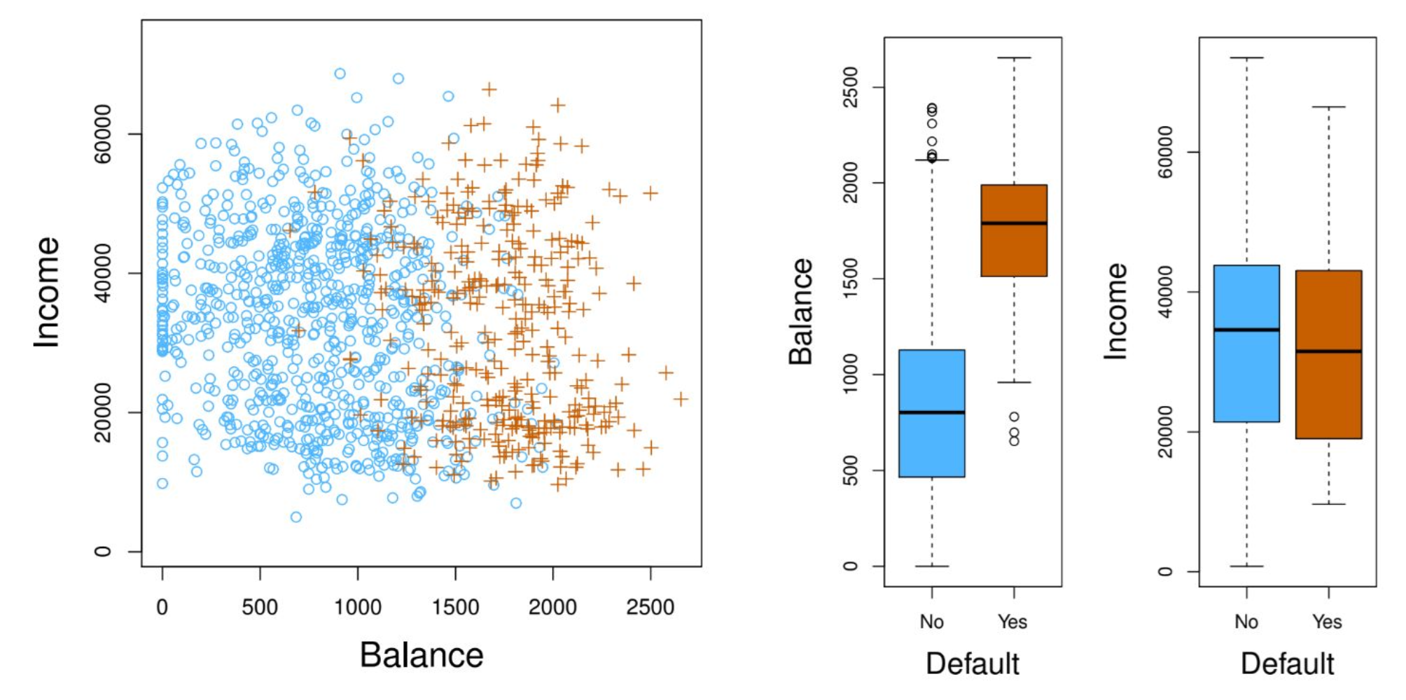
LDA 모델을 Credit Card 데이터에 돌린 confusion matrix:

	True No	True Yes	Total
Pred No	9644	252	9896
Pred Yes	23	81	104
Total	9667	333	10000

Misclassification rate: $(23 + 252) / 10000 = 2.75%$
근데 모든 observation을 No로만 분류하는 trivial classifier도 $333/10000 = 3.33%$밖에 안 됨.

즉, overall accuracy만 보면 모델이 별로 안 좋아 보임. 더 자세히 보자.

Error Types

	True No	True Yes
Pred No	TN	FN
Pred Yes	FP	TP

False positive rate $\dfrac{\mathrm{FP}}{\mathrm{FP}+\mathrm{TN}}$: 음성을 양성으로 잘못 분류한 비율. 예시에서 $23/9667 = 0.2%$.
False negative rate $\dfrac{\mathrm{FN}}{\mathrm{TP}+\mathrm{FN}}$: 양성을 음성으로 잘못 분류한 비율. 예시에서 $252/333 = 75.7%$. 엄청 높음.

Credit card default 예측에서 default인 사람을 못 잡으면 큰 손실이니까 FN이 critical.

은행 입장에서 고객이 {돈을 못 갚을 줄 알았는데 알고 보니 갚을 능력이 있었다}는 케이스보다 {돈을 갚을 줄 알았는데 못 갚는다}는 상황이 더 critical (이미 돈은 빌려줬는데)
그런데 75.7%면 거의 못 잡고 있는 셈.

Threshold 조정

위 confusion matrix는 $p(\text{Default} = \text{Yes} | \text{Balance}, \text{Student}) \geq 0.5$ 기준임. threshold를 0.5에서 다른 값 $\tau \in [0, 1]$로 바꾸면 error rate가 달라짐:

\[\hat{y} = \text{Yes} \iff p(\text{Default} = \text{Yes} \| \text{Balance}, \text{Student}) \geq \tau\]

threshold를 0.5에서 더 낮춰서 0.1 같은 값으로 내리면 FN이 줄어들지만 FP가 늘어남. Overall error rate는 오히려 증가할 수도 있음.

즉, 단일 threshold만으로 모델을 평가하는 건 적절하지 않음. trade-off가 존재.

ROC Curve

ROC (Receiver Operating Characteristic) curve는 threshold를 0부터 1까지 쭉 바꿔가며 False positive rate vs. True positive rate ($= 1 - \mathrm{FNR}$)를 한꺼번에 보여줌.

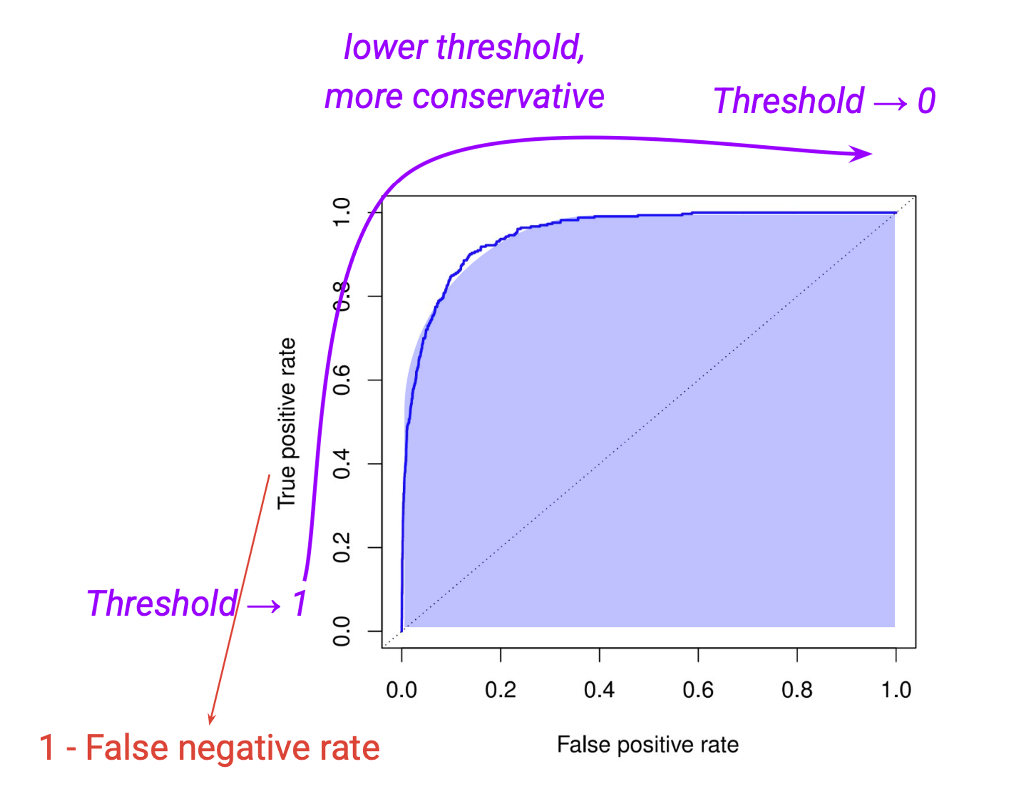
AUC (Area Under the Curve)가 종합 성능 지표로 널리 쓰임.
AUC 높을수록 좋은 모델.
threshold $\to 0$이면 모든 걸 positive로 → TPR $\to 1$, FPR $\to 1$ (오른쪽 위)
threshold $\to 1$이면 모든 걸 negative로 → TPR $\to 0$, FPR $\to 0$ (왼쪽 아래)
곡선이 왼쪽 위 모서리에 가까울수록 좋음.

Naive Bayes

핵심 가정

Naive Bayes는 generative classifier의 한 종류인데, $\mathbf{x} \in \mathbb{R}^d$에 대해 다음을 가정함:

\[p(\mathbf{x}|\mathbf{y}) = \prod_{j=1}^{d} p(x_j | \mathbf{y})\]

라벨이 주어졌을 때 $\mathbf{x}$의 각 원소가 서로 독립 (conditional independence) 이라고 가정

가정이 비현실적인 이유

이미지에서 “꽃” 클래스가 주어졌을 때 두 픽셀이 독립일 리 없음. 인접 픽셀은 거의 비슷한 색.
텍스트에서 단어 vector의 각 dimension(단어)이 독립일 리 없음. “the red dog”에서 dog가 있으면 red도 같이 나올 확률이 높음.

거의 항상 highly dependent. 그럼에도 불구하고 Naive Bayes는 놀랍게도 잘 작동함.

왜 잘 작동하는가?

텍스트 분류 {tech, politics}로 예시:

“Open AI is developing the next version of ChatGPT with 10x larger parameters.”

“President Biden and former President Trump are running for 2024 election.”

이 단어들이 이 문장에 등장하게 된 건 우연이 아님. 맥락이 있고 문법이 있으니 존재. IID를 가정할 수 없지만 일단 계산해봐
각 문장의 각 단어들에 대해서 $p(x|\mathbf{y}=\text{tech})$, $p(x|\mathbf{y}=\text{politics})$ 를 둘 다 계산해 봐
절대적인 확률은 말도 안 되는 낮은 확률이 나오겠지만, 굳이 비교를 하자면, 위 단어들은 $p(x|\mathbf{y}=\text{tech})$가 높고, 아래 단어들은 $p(x|\mathbf{y}=\text{politics})$가 높음.
sentence-level probability $p(\mathbf{x}|\mathbf{y})$는 word-level 확률의 곱과는 실제로 거리가 멀지만, 같은 $\mathbf{x}$에 대해 $p(\mathbf{x}|\mathbf{y}=\text{tech})$와 $p(\mathbf{x}|\mathbf{y}=\text{politics})$의 relative order는 보통 안 바뀜.
분류 자체는 그 순서만 맞으면 되니까 잘 동작하는 것.

Weather 데이터 예시

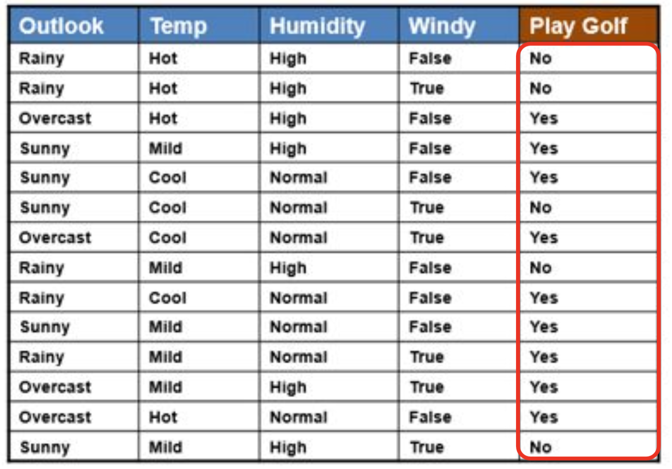
훈련 데이터에서:

$p(\text{Play Golf} = \text{yes}) = 9/14$
$p(\text{Play Golf} = \text{no}) = 5/14$

질문: $\mathbf{x} = $ {Outlook=sunny, Temp=Hot, Humidity=High, Windy=False} 일 때 골프 칠 것인가?

$p(\mathbf{y}|\mathbf{x}) \propto p(\mathbf{x}|\mathbf{y}) * p(\mathbf{y})$이고, Naive Bayes 가정으로 $p(\mathbf{x}|\mathbf{y}) = \prod_j p(x_j|\mathbf{y})$.

yes일 확률:

\[p(\mathbf{x} \| \text{yes}) = p(\text{sunny}\|\text{yes}) \cdot p(\text{Hot}\|\text{yes}) \cdot p(\text{High}\|\text{yes}) \cdot p(\text{False}\|\text{yes})\] \[= \frac{3}{9} \cdot \frac{2}{9} \cdot \frac{3}{9} \cdot \frac{6}{9} = \frac{3 \cdot 2 \cdot 3 \cdot 6}{9 \cdot 9 \cdot 9 \cdot 9} = 0.016\] \[p(\text{yes} \| \mathbf{x}) \propto p(\text{yes}) \cdot p(\mathbf{x}\|\text{yes}) = \frac{9}{14} \cdot 0.016 = 0.013\]

no일 확률:

\[p(\mathbf{x} \| \text{no}) = p(\text{sunny}\|\text{no}) \cdot p(\text{Hot}\|\text{no}) \cdot p(\text{High}\|\text{no}) \cdot p(\text{False}\|\text{no})\] \[= \frac{2}{5} \cdot \frac{2}{5} \cdot \frac{4}{5} \cdot \frac{2}{5} = 0.051\] \[p(\text{no} \| \mathbf{x}) \propto p(\text{no}) \cdot p(\mathbf{x}\|\text{no}) = \frac{5}{14} \cdot 0.051 = 0.018\]

$0.018 > 0.013$이니까 최종 예측은 no. 골프 안 침.

실전에서의 문제점

Zero-frequency problem

훈련 데이터에서 어떤 변수가 한 번도 안 나왔으면 $p(x_j|\mathbf{y}) = 0$.
Conditional independence 가정 때문에 곱의 형태라, 하나라도 0이면 전체 $p(\mathbf{x}|\mathbf{y}) = 0$이 됨:

\[p(\mathbf{x}\|\mathbf{y}) = \prod_{j=1}^{d} p(x_j\|\mathbf{y}) = 0 \quad \text{if } \exists j: p(x_j\|\mathbf{y}) = 0\]

해결법: 모든 가능한 event에 작은 확률 $\varepsilon$를 더해줌 (smoothing, 예: Laplace smoothing).

Numerical issue

$d$가 적당히만 커도 확률의 곱이 underflow 날 정도로 작아짐. 그래서 곱 대신 log를 씌워서 합으로 계산:

\[\log p(\mathbf{x}\|\mathbf{y}) = \log \prod_{j=1}^{d} p(x_j \| \mathbf{y}) = \sum_{j=1}^{d} \log p(x_j \| \mathbf{y})\]

이건 거의 표준 practice.

정리

Bayes Classifier: risk를 최소화하는 optimal classifier. posterior $p(\mathbf{y}|\mathbf{x})$ 비교로 분류.
Discriminant Analysis
$p(\mathbf{x}|\mathbf{y})$를 Gaussian으로 가정한 generative approach.
- LDA: 공분산 같다고 가정 → linear boundary
- QDA: 공분산 다를 수 있음 → quadratic boundary
평가 지표: accuracy 하나로는 부족. FP/FN trade-off가 있고, ROC와 AUC로 종합 평가.
Naive Bayes: $p(\mathbf{x}|\mathbf{y}) = \prod p(x_j|\mathbf{y})$. 가정은 비현실적이지만 실제로 잘 작동함. zero-frequency와 numerical underflow는 smoothing과 log로 해결.

AI, ML

This post is licensed under CC BY 4.0 by the author.