[paper summary] Bao: Making Learned Query Optimization Practical

Posted Jul 1, 2025 Updated Jul 14, 2025

By Jina Kim 14 min read

Summary

Bao (Bandit optimizer) is a novel learned query optimization system that addresses the practical limitations of previous machine learning approaches to database query optimization.

Key Problems with Existing ML Query Optimizers

Long training time - Most ML techniques require impractical amounts of training data
Inability to adapt - Cannot handle changes in workload, data, or schema
Tail catastrophe - Can perform catastrophically poorly on some queries (100x regression)
Black-box decisions - Difficult to understand or debug
Integration cost - Hard to integrate into real database systems

Bao’s Approach

Instead of learning a query optimizer from scratch, Bao:

Takes an existing optimizer (e.g., PostgreSQL) and learns when to activate/deactivate specific features
Uses query hints to guide the traditional optimizer on a per-query basis
Combines Tree Convolutional Neural Networks (TCNN) with Thompson sampling (contextual multi-armed bandit)
Treats each hint set as an “arm” in the bandit problem

Key Advantages

Short training time - Can outperform traditional optimizers in ~1 hour vs. days for other approaches
Robust to changes - Adapts to workload, data, and schema changes by leveraging traditional optimizer’s estimates
Better tail latency - Improves worst-case query performance significantly
Interpretable - Decisions can be inspected and Bao can be enabled/disabled per query
Low integration cost - Easy to integrate as PostgreSQL extension without code changes
Extensible - Can add new query hints without retraining

Experimental Results

~50% improvement in cost and latency over PostgreSQL across multiple workloads
~20% improvement over commercial database system
Significant tail latency reductions (e.g., 99% latency from 130s to <20s)
Maintains performance even with dynamic workloads and schema changes
Converges within 2-3 hours compared to 24+ hours for other learned optimizers

Technical Details

Uses 48 hint sets covering different combinations of join operators and scan operators
Vectorizes query plans using operator encoding, cardinality estimates, and optional cache information
Retrains model every n queries (default: 100) using k most recent experiences (default: 2000)
Available as open-source PostgreSQL extension

Bao represents the first practical learned query optimizer that successfully addresses the fundamental challenges preventing adoption of ML techniques in real database systems.

Details

1. Introduction

Previous research on query optimization using machine learning had the following problems:

Long training time
Inability to adjust to workload changes
Tail catastrophe
Black-box decisions
Integration cost

Bao (Bandit optimizer) leverages information from existing optimizers and sits on top of the optimizer rather than replacing it, providing the following advantages:

Short training time
Robustness to schema, data, and workload changes
Better tail latency
Interpretability and easier debugging
Low integration cost
Extensibility

Bao also has disadvantages:

Query optimization time increases
Limited set of hints restricts the action space. Even if hints outside the action space might be optimal, they cannot be learned.

Key contributions:

Introduce Bao, a learned system for query optimization that is capable of learning how to apply query hints on a case-by-case basis
Bao outperforms both open source and commercial systems in cost and latency, while adapting to changes in workload, data, and schema

2. Methodology Overview

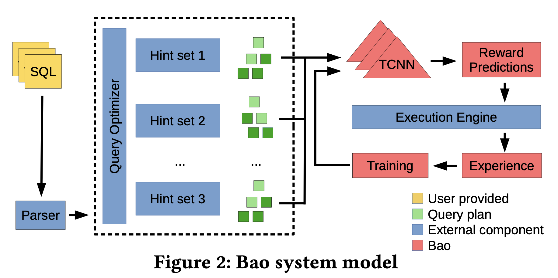
When a query arrives

  
 query = "SELECT * FROM ..."
 hint_sets = [hint_set1, hint_set2, ..., hint_set_n]  # 48 candidates

The basic optimizer generates plans for each hint set (number of generated plans is configurable)

  
 plans = []
 for hint_set in hint_sets:
     plan = postgres_optimizer.generate_plan(query, hint_set)
     plans.append(plan)

Sample θ from experience using Thompson Sampling

  
 θ_sampled = sample_theta_from_posterior(experience)

Predict performance for each plan

  
 predictions = []
 for plan in plans:
     pred = model(plan, θ_sampled)  # Predict all plans with the same θ
     predictions.append(pred)

Select hint set with best predicted performance

  
 best_hint_set = hint_sets[argmin(predictions)]

Add actual execution performance to experience

3. Selecting Query Hints

3.1. Structure

3.1.1. Assumptions and Definitions

Modeling hint set as query optimizer

Bao models each hint set $HSet_i ∈ F$ as a query optimizer function:$HSet_i: Q → T$

$q \in Q$: Query space
$t \in T$ : Query plan tree space
$HSet_i$: Function that takes query q and returns query plan tree t
Pass query Q and selected $HSet_i$ to the optimizer to receive plan tree for each hint
Each query plan tree $t ∈ T$ consists of arbitrary number of operators
- Selected from known finite operator set
- Trees can be arbitrarily large but operator types are predetermined

Selection Function: $B: Q → F$

$B$: Decides which hint set to use given query $q$
Bao’s goal: Select hint set that generates the best query plan

Performance Metric Definition

$P$: User-defined performance metric
- Execution time, disk I/O count, etc.
- Measures query plan quality using this metric

3.1.2. Formulation as Regret Minimization Problem

\[R_q = {(P(B(q)(q)) - \min_{i} P(HSet_i(q)))}^2\]

$R_q$: Regret (performance difference) for query q
$P(B(q)(q))$: Performance of plan created with Bao’s selected hint set
- $B(q)(q)$ : Apply selected hint set($B(q)$) to query $q$
$\min P(HSet_i(q))$: Optimal performance among all hint sets

3.1.3. Contextual Multi-Armed Bandits (CMABs)

Multi-Armed Bandit Problem

Agent: Entity that must make repeated choices
Arms: Fixed number of options
Context: Situational information given each time
Reward: Reward received after selection

Operation process:

Agent receives contextual information
Selects one of several arms
Receives payout (reward)
Receives new context and selects again
Each trial is considered independent

Goal: Maximize reward (i.e., minimize regret)

Multi-Armed Bandit Problem in Bao

Arms ↔ Hint Sets:
- Each hint set is one arm
Context ↔ Query Plans:
- Context: Set of query plans generated by existing optimizer with each hint set
- Agent (Bao) sees all possible query plans and selects one
Reward ↔ Performance:
- Performance result of executing selected query plan becomes reward
- E.g., inverse of execution time, inverse of I/O count, etc.

Operation process in Bao:

Query $q$ arrives
Generate query plan for each hint set $HSet_i$: $t_i = HSet_i(q)$
Context = ${t_1, t_2, …, t_n}$ (all generated query plans)
Bao selects one of these plans
Execute selected plan and observe performance
Add (plan, performance) pair to experience

3.1.4. Thompson Sampling

Use Thompson sampling for regret minimization of contextual multi-armed bandit

General ML vs. Thompson Sampling

General ML

θ* = argmax P(θ|E)  // Select only the most likely parameter
prediction = model(query, θ*)  // Always predict with the same θ*

Thompson sampling

Thompson sampling operates while accumulating experience

Learn predictive model using experience

$E$ = [(plan1, actual_performance1), (plan2, actual_performance2), …]

θ_sampled ~ P(θ|E)  // Sample θ from probability distribution
prediction = model(query, θ_sampled)  // Predict with different θ each time

Sample parameter theta from distribution given $E$(experience)
- Generate slightly different models trained on the same data

To recommend hint sets, we need performance prediction values for each hint set candidate.
Use performance estimation model $M_{\theta}$:

Input : plan tree
Output : estimated performance
Model parameter $\theta$

# Random sampling with replacement from experience each time
bootstrap_data = random_sample_with_replacement(E, size=1000)
θ_new = train_neural_network(bootstrap_data)

Sample actual performance values from experience
Extract $\theta$ by training model on sampled data

Different $\theta$ emerges each time because sampled data differs
When data is scarce: Various $θ$s are sampled → exploration
- With little data, $P(θ|E)$ has high variance → diverse $θ$ sampling
- Outliers are more likely to appear distinctly
When data is abundant: Similar $θ$s are sampled → exploitation
- Sampling from large dataset preserves most patterns
- With abundant data, $P(θ|E)$ has low variance → similar $θ$ sampling

With extracted $θ$, predict performance for all hint sets using the same sampled $θ$ Execute using hint with best predicted performance

3.2. Predictive model $M_{\theta}$ architecture

The core of Thompson Sampling is a model that predicts query plan performance. Bao uses Tree Convolutional Neural Network (TCNN) for this purpose.

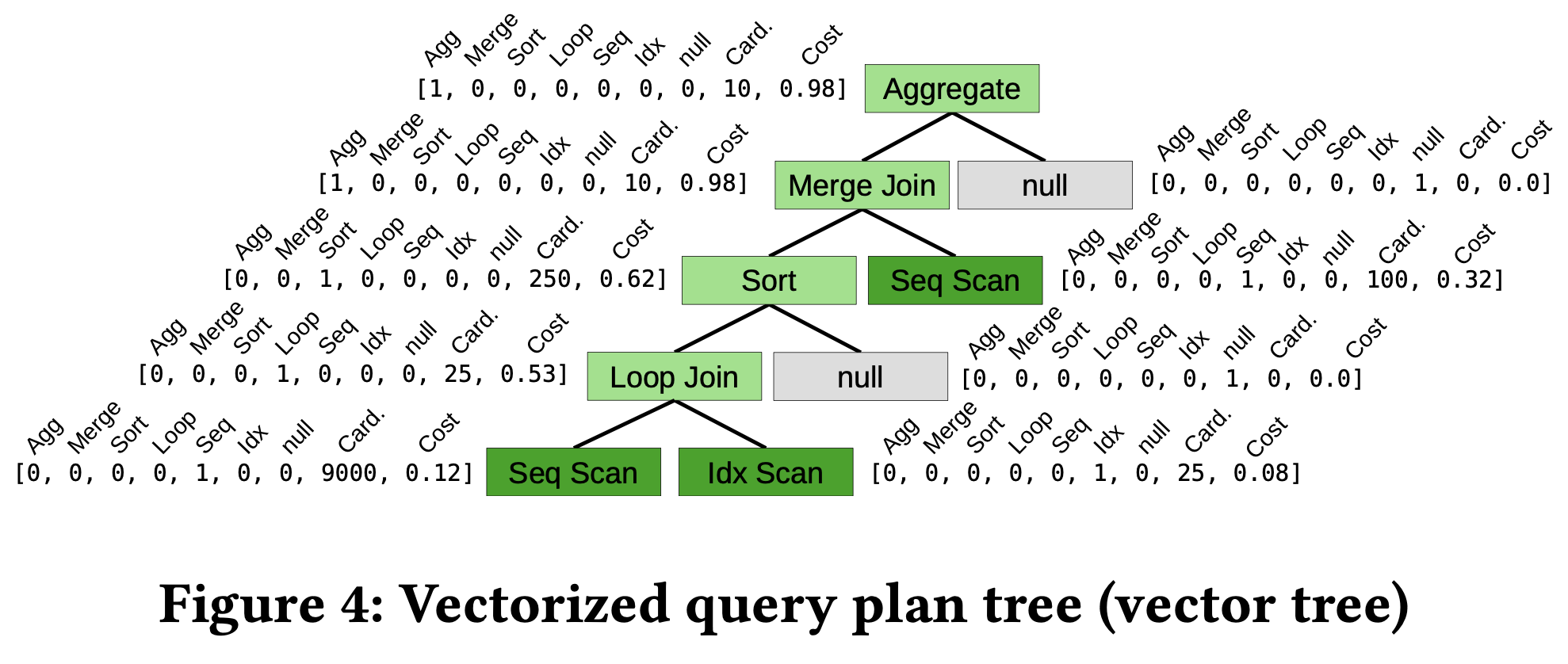
3.2.1. Vectorizing query plan trees

Binarization

Problem: Many queries include non-binary operations

Aggregation, Sorting can only have 0 or 1 child
Tree convolution is more efficient on strictly binary trees

Solution: Convert non-binary tree to binary tree

Original:                    Binarized:
   Aggregate                    Aggregate
   |                           /        \
   Merge Join              Merge Join   null
   |                       /        \
   Sort                   Sort      null

Single child: Add “null” node on the right
Multiple children: Split into left-deep tree

Vectorization

Convert each node to a vector:

One-hot encoding of operator:

 [1,0,0,0,0,0,0, ...] = Aggregate
 [0,1,0,0,0,0,0, ...] = Merge Join
 [0,0,1,0,0,0,0, ...] = Sort

Cardinality and Cost information:
1 [..., cardinality_estimate, cost_estimate]
- Estimates provided by PostgreSQL optimizer
Cache information (optional):
1 [..., cache_hit_ratio]
- Cache data ratio for scan nodes
- E.g., 0.32 = 32% is in cache

Final vector example:

[1,0,0,0,0,0,0, 10, 0.98] = Aggregate, card=10, cost=0.98
[0,1,0,0,0,0,0, 250, 0.62] = Merge Join, card=250, cost=0.62

Advantages of Vectorization

Schema-agnostic:
- Does not directly include table/column names
- No need to start from scratch when schema changes
Data change adaptability:
- Cardinality/cost estimates are automatically updated by PostgreSQL
- Data changes are naturally reflected

3.2.2. Tree convolutional neural networks

Intuition behind Tree Convolution

Human Expert Pattern Recognition:

“Merge joins pipeline without intermediate sorts” → good performance
“Hash join over very large relation” → spill risk
“Merge join on top of hash join” → unnecessary sort

Purpose of Tree Convolution:

Automatically learn these structural patterns
Recognize good and bad patterns in query plan trees

TCNN Architecture

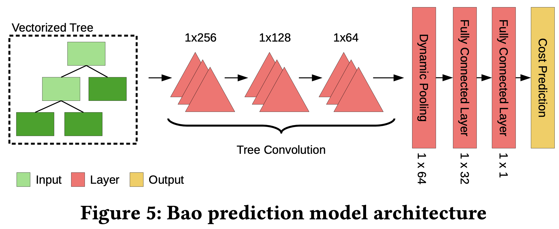
Tree Convolution Layers (3 layers):
- Tree-shaped “filters” scan through query plan tree
- Each layer learns more complex patterns
- Layer 1: Simple operator pairs (hash join + hash join)
- Layers 2-3: Complex structures (long chain of merge joins)
Dynamic Pooling:
- Flatten tree structure to single vector
- Fixed-size output regardless of tree size
Fully Connected Layers:
- Pooled vector → performance prediction
Activation & Normalization:
- ReLU activation functions
- Layer normalization

Inductive Bias

Why tree convolution is suitable for query optimization:

Specialized for structural pattern recognition
Naturally matches hierarchical characteristics of query plans
More effective than simple fully-connected networks

Thompson Sampling

General ML: Find most likely model parameters

$E[P(θ|E)]$ (modal parameters)

Thompson Sampling: Probabilistically sample parameters

Sample from $P(θ|E)$ distribution
Balance exploration vs exploitation

Bao’s Choice: Bootstrap Sampling

Sampling with replacement of $|E|$ items from experience $E$
Train neural network with bootstrapped data
The resulting $θ$ corresponds to a sample from $P(θ|E)$

3.3. Training Loop

3.3.1. Experience Control

Second, instead of allowing $|𝐸|$ to grow unbounded, we only store the 𝑘 most recent experiences in 𝐸.

Train model using stored experience data to extract parameters. As experience size grows, model training cost increases significantly

Experience E maintains only recent k items (sliding window)
When new experience arrives, remove the oldest one

3.3.2. Model Retraining Method

By far the simplest technique, which has been shown to work well in practice [63], is to train the neural network as usual, but on a “bootstrap” [15] of the training data: the network is trained using $|𝐸|$ random samples drawn with replacement from 𝐸.

Perform bootstrap sampling from all current data in E (k items)
Train neural network with bootstrapped data to obtain new θ
Draw $|E|$ samples with replacement for training (i.e., sampling with replacement k items from k items)

3.3.3. Retraining Frequency

Instead of resampling the model parameters (i.e., retraining the neural network) after every query, we only resample the parameters every 𝑛th query.

Retrain model every nth query
Set n=100 in experiments

3.3.4. Model Optimization

Can trade off model quality and training overhead by changing k and n values
Since database query execution mainly uses CPU while model training uses GPU, when training the model, the training layer can be separated to GPU for training, and once training is complete, the model can be attached to the database.

4. Experiments

4.1. Settings

4.1.1. Datasets

Dataset	Size	Queries	Workload	Data	Schema
IMDb	7.2 GB	5000	Dynamic	Static	Static
Stack	100 GB	5000	Dynamic	Dynamic	Static
Corp	1 TB	2000	Dynamic	Static	Dynamic

Dataset Characteristics:

IMDb: Join Order Benchmark extension, introduces new query templates over time
Stack: Real StackExchange data, simulates data drift by monthly data loading
Corp: Anonymous corporate dashboard workload, schema normalization after 1000th query

4.1.2. Experimental Environment

Cloud: Google Cloud Platform N1-4 VM + TESLA T4 GPU
On-premise: 4 CPU cores, 15GB RAM, Intel Xeon Gold 6230, NVIDIA Tesla T4
Evaluation: Time series split method (train on past data only, predict future queries)

4.1.3. Model Configuration

Architecture: 3-layer tree convolution + dynamic pooling + 2 fully connected layers
Training: Adam optimizer, batch size 16, 100 epochs or convergence
Parameters: 48 hint sets, window size k=2000, retrain every n=100 queries

4.1.4. Workload Characteristics

Median latency: 280ms (IMDb), 310ms (Stack), 520ms (Corp)
95th percentile: 21s (IMDb), 28s (Stack), 3m (Corp)
Pareto distribution: 80% execution time concentrated in 20% queries (18%, 23%, 21%)

4.2. Baselines

1. PostgreSQL

Default PostgreSQL optimizer
Retuned for each hardware platform
Applied standard configuration and best practices

2. Commercial System (ComSys)

Commercial database system
Configuration verified by professional consultant
Configured and tuned according to documentation and best practices
License costs excluded from measurement

3. Prior Learned Optimizers

Neo: Uses tree convolution, generates complete query plans
DQ: Deep Q-learning, hand-crafted features + FCNN

4.3. Results

4.3.1. Practicality Results

Cost and Performance (Google Cloud N1-16)

vs PostgreSQL: ~50% cost and latency reduction (all datasets)
vs ComSys: ~20% cost and latency reduction
Results include GPU attachment costs
Cost impact factors: Execution time reduction by Bao »> optimization/GPU time increase
Dramatic improvements in tail latency have significant impact

Hardware Scaling (IMDb workload)

Larger VMs show greater Bao improvement effects (vs PostgreSQL)
ComSys adapts better to hardware changes

Tail Latency Improvements

99% latency: 130 seconds → under 20 seconds (PostgreSQL, N1-8)
Significant tail latency reduction across all VM types
Median performance improvement is minimal (<5%)

Training Time & Convergence

PostgreSQL: Exceeds performance after ~2 hours
ComSys: Exceeds performance after ~3 hours
Stable adaptation to dynamic workload changes

Query Regression Analysis

Only 3 regressions out of 113 JOB queries (all under 3 seconds)
10 queries show over 20-second improvements

Optimization Time

PostgreSQL: Maximum 140ms
ComSys: Maximum 165ms
Bao: Maximum 230ms (70ms increase, utilizes parallel processing)

4.3.2. Hint Analysis Results

Best Hint Sets (Top 5 responsible for 93% improvement)

Disable nested loop join (35%)
Disable index scan & merge join (22%)
Disable nested loop + merge + index scan (16%)
Disable hash join (10%)
Disable merge join (10%)

Query Plan Impact

4271/5000 queries selected different operators
3792/5000 queries selected different access paths
2110/5000 queries selected different join orders

4.3.3. (Ablation) ML Model Results

Model Comparison (First 2000 queries)

Bao (TCNN): Best performance
Random Forest: Significantly lower performance
Linear Regression: Very low performance
Demonstrates necessity of complex tree convolution models

Model Accuracy

Initial Q-error: 3 (relatively inaccurate)
Even with inaccuracy, prevents catastrophic plan selection

Prior Learned Optimizers vs Bao

Stable workload: Neo surpasses Bao after 65 hours, 15% better after 200 hours
Dynamic workload: Both Neo and DQ fail to surpass Bao within 72 hours
Bao excels in fast convergence and dynamic adaptability

GPU Training Time

Window size 2000: ~1 minute
Window size 5000: ~3 minutes
Cloud environment variability exists

5. PostgreSQL Integration

5.1. Key Features/Implementation

Utilizing Hooks System

Extends functionality using PostgreSQL’s hooks system
Easy integration into existing PostgreSQL instances without code recompilation
Adds new functionality based on function pointers

Per-query Activation

  
SET enable_bao TO [on/off]

Enable/disable Bao per query
For short execution time queries, optimization time may exceed execution time
Preserves existing work by disabling on queries already manually tuned by DBAs

Active vs. Advisor Mode

Active mode: Bao automatically selects hint sets and learns from performance
Advisor mode:
- Query optimization using PostgreSQL planner only
- Observes performance of executed queries and trains predictive model
- Provides 3 additional pieces of information during EXPLAIN queries:
  1. Expected performance of generated query plan
  2. Hint set recommended by Bao
  3. Expected performance improvement from that hint set

Triggered Exploration

Can mark performance-critical queries as “critical”
Critical queries are periodically executed with all hint sets to collect performance data
Critical experiences receive higher weights during predictive model retraining
Prevents performance regression on critical queries, ensuring optimal performance

Database

This post is licensed under CC BY 4.0 by the author.