[paper summary] Balsa: Learning a Query Optimizer Without Expert Demonstrations

Summary

Balsa is the first learned query optimizer that can match or exceed expert optimizer performance without learning from existing expert optimizers or demonstrations.

Key Problems with Existing Approaches

1. High development cost - Expert optimizers take months to write and years to refine
2. Dependency on expert systems - Previous learned optimizers (DQ, Neo) require mature optimizers or expert cost models to bootstrap from
3. Disastrous plan problem - Most execution plans are orders of magnitude slower than optimal, hindering learning progress
4. Limited applicability - Cannot be applied to new systems where expert optimizers don’t exist

Balsa’s Approach

Uses a “Bootstrap, Safely Execute, Safely Explore” methodology:

1. Simulation Learning - Bootstraps from a minimal cost model (sum of estimated result sizes) to learn basic knowledge quickly
2. Safe Execution - Uses adaptive timeouts and transfers to real execution environment safely
3. Safe Exploration - Explores within “trust regions” of top-k plans rather than random exploration
4. Diversified Experiences - Merges experiences from multiple agents to improve generalization

Key Advantages

1. No expert dependency - First approach to learn query optimization without expert demonstrations
2. Novel safety mechanisms - Timeout policies and safe exploration prevent learning from getting stuck on slow plans
3. Superior generalization - Better robustness on unseen queries compared to expert-dependent methods
4. Practical efficiency - Matches expert performance in 1.4-2.5 hours, reaches peak in 4-5 hours

Experimental Results

• PostgreSQL: 2.1× speedup on training queries, 1.7× on test queries
• Commercial DB: Up to 2.8× speedup on training, 1.9× on test queries
• Outperforms Neo (expert-dependent method): 9.6× faster training with better generalization
• Data efficiency: Needs only 3.2K-7.4K plan executions to match expert performance
• Maintains stable performance while previous methods suffer high variance on unseen queries

Balsa opens the possibility of automatically learning query optimizers for future computing environments where expert-designed optimizers don’t exist, significantly reducing the human development cost for new database systems.

---

Details

1. Introduction

Research Background and Problems

• Query Optimizer Development Cost: Experts take months to create the first version and years to achieve completeness
• Limitations of Existing Systems: PostgreSQL has been continuously optimized for over 20 years, Spark SQL (2014) only added CBO in 2017, CockroachDB completed CBO after 9 months of intensive effort
• Key Question: Can machine learning learn query optimization without the help of existing expert optimizers?

Differences from Previous Research

• Previous Research (DQ, Neo)
  • DQ: Learns from expert optimizer’s cost model
  • Neo: Learns from expert optimizer’s plans and actual execution results
  • Commonality: All depend on existing expert optimizers
• Balsa’s Innovation
  • First to learn without expert optimizer. Learns query optimization purely through reinforcement learning without help from expert optimizer
  • Can automatically learn optimization even in environments where expert optimizers do not exist for new data systems

Key contributions:

1. introduce Balsa, a learned query optimizer that does not learn from an existing, expert optimizer.
2. Simulation-to-Reality Learning:
   • Learn basic knowledge in simulator then safely learn in real environment
   • Proceed with learning while avoiding catastrophic plans
3. Safe Execution with Timeouts:
   • Early termination of slow plans through time limits
   • Prevent unpredictable learning interruptions
4. Safe Exploration:
   • Safe exploration among “probably good” plans instead of random search
   • Prioritize execution of unexplored plans with count-based exploration
5. Diversified Experiences:
   • Merge experiences from multiple independently trained agents
   • Improve generalization performance
6. Balsa can outperform both an open-source (PostgreSQL) and a commercial query optimizer, after a few hours of training.
7. despite not learning from an expert optimizer, Balsa outperforms the prior state-of-the-art technique that does.

---

2. Methodology Overview

Classical Design vs Balsa Approach

Classical Design

Cost Model: C : plan → cost

• Uses cost model implemented by experts
• Estimates immediate cost of plans
• Enumerates candidate plans with dynamic programming (DP) and scores them with cost model

Balsa Approach (RL Approach)

Value Function: V : (query, plan) → overall cost or latency

• Value function estimates total cost/latency of entire query when using subplan
• Directly optimizes final objective (overall latency) rather than immediate cost

---

Concrete Operation Example

For query Q joining tables {A, B, C, D}:

Step 1: Select first join

{A, B, C, D} ⇒ [V(Q, A⋈B); V(Q, A⋈C); ...]

Compare values of all possible 2-table joins to select optimal first join

Step 2: Select second join

If A⋈C is optimal:

{A⋈C, B, D} ⇒ [V(Q, B⋈D); V(Q, B⋈(A⋈C)); ...]

---

Learned Value Network

PostgreSQL Cost Model  →  V_sim  →  V_real  →  Optimized Plans
       (Teacher)        (Student) (Fine-tuned)  (Final Output)

Simulation Phase: Learn basic knowledge with minimal cost model

• Build dataset by estimating costs for all possible plans found by Dynamic Programming using PostgreSQL’s cardinality estimator (minimal model that doesn’t consider physical operators or execution engine characteristics)
• Train value network $V_{sim}$ that receives (query, plan) and predicts cost using this dataset

Real Execution Phase: Fine-tune value network with actual query execution

• Develop prediction model $V$ by actually executing queries
• Initialize $V_{real} \leftarrow V_{sim}$
• Repeat the following steps:
  1. Use current $V_{real}$ to optimize new unseen query -> generate plan -> execute -> measure latency -> store latency
  2. Update $V_{real}$ with collected (query, plan, latency) data

---

3. Bootstrapping from Simulation

Need for Simulation Bootstrapping

Disastrous execution plan

• Since db’s search space is vast, poor execution plans can be created
• Waiting for disastrous execution plans stops learning
  • <-> AI learning games receives immediate feedback when making bad moves and games end quickly = can learn more rounds as games end quickly
  • Bad execution plans in db take long time = takes long to receive feedback that it’s a bad plan, reducing time to learn other queries
• Learning with existing cost models can reduce disastrous execution plans
  • Not learning expert optimizer. Learning cost predictions of cardinality estimator

Minimal Simulator

Advantages of minimal simulator:

• Usable with any engine (doesn’t model physical details)
• Requires only minimal prior knowledge
• Purpose is to avoid catastrophic plans (not expert-level performance)

Disadvantages:

• Inaccuracy: Inherently inaccurate model
• Needs fine-tuning in real execution phase to compensate

Simulation Data Collection

$V_{sim}$ learns (query, plan, cost) dataset to avoid disastrous execution plans. The (query, plan, cost) dataset was generated as follows.

Plan Enumeration through Dynamic Programming

1. Execute Selinger’s bottom-up DP for each training query
2. Start with 2-table joins and gradually expand (3-table, 4-table, … add one table at a time to intermediate states)
3. Obtain cost estimate C for each enumerated plan T
4. Generate data point: (query=T, plan=T, overall cost=C)

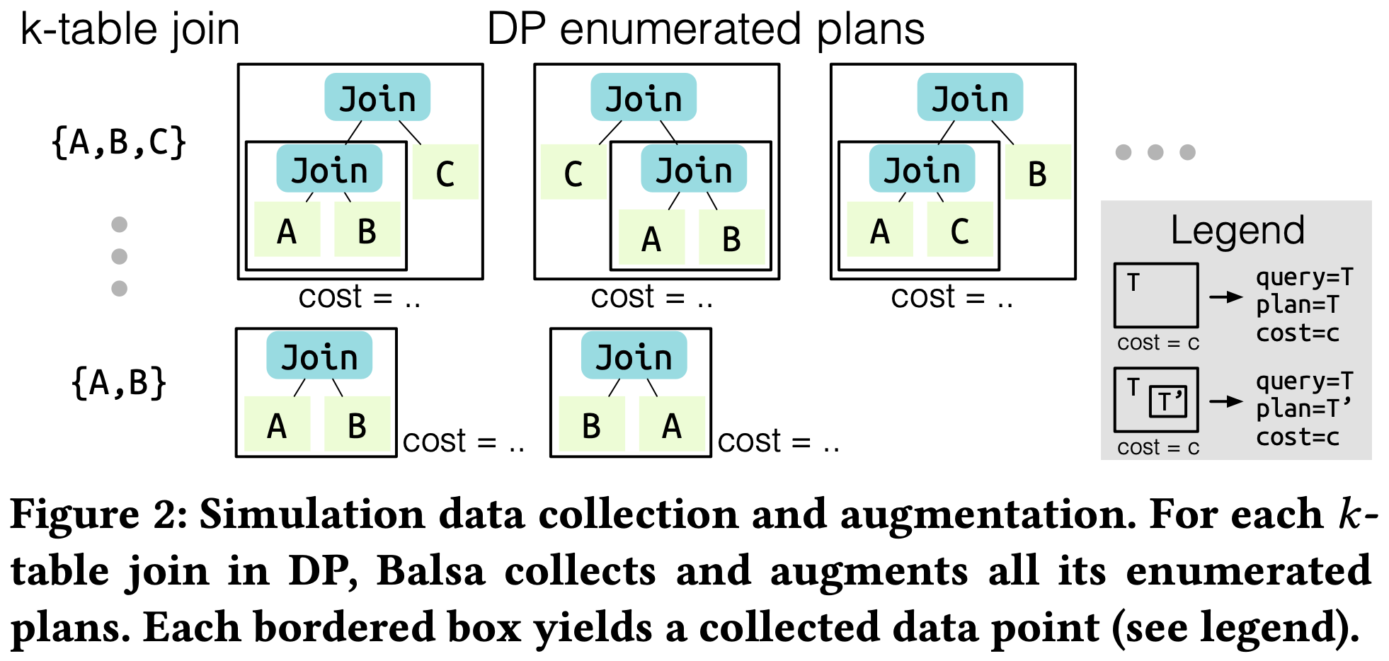
• Collect all plans enumerated by DP for k-table joins
• Each bordered box becomes one collected data point

Data Augmentation

Using technique proposed by DQ:

{(query=T, plan=T', overall cost=C) : ∀T' ⊆ T}

Given (query=T, plan=T, cost=C)

• Generate data points with same cost C for all subplans T’ of T

• Significantly increase dataset quantity and diversity

• All states (subplans) of trajectory (entire query/final plan) share same reward
• Intermediate rewards are 0 and terminal rewards are negative costs of final plans

Using Cout Cost Model

$V_{sim}$ is trained on dataset consisting of (query, plan, cost). When calculating the “cost” part for each plan in simulation dataset, the following cost model is used.

Cout(T) = {
  |T|                           if T is a table/selection
  |T| + Cout(T1) + Cout(T2)     if T = T1 ⋈ T2
}

• “Fewer tuples lead to better plans”
• Simply sums estimated result sizes of all operators
• No prior knowledge about physical operators or execution engine

ex)

Cout((A ⋈ B) ⋈ C) = |((A ⋈ B) ⋈ C)| + Cout(A ⋈ B) + Cout(C)
                   = |((A ⋈ B) ⋈ C)| + |A ⋈ B| + Cout(A) + Cout(B) + |C|
                   = |((A ⋈ B) ⋈ C)| + |A ⋈ B| + |A| + |B| + |C|

Simulator Components

Simulator = Cout model + Cardinality estimator

1. Cout model: Formula for calculating plan costs
2. Cardinality estimator: Provides $|T|$ values (PostgreSQL’s histogram-based estimator)

Learning Objective of $V_{sim}$

= “Mimic” the Cout model

V_sim(query, plan) ≈ Cout(plan)

V_sim is a neural network:

• Can learn complex patterns beyond simple formulas
• Has generalization capability
• Can be fine-tuned later with real execution data

---

4. Learning from real execution

Simulation is rough learning with imperfect cost model to avoid only disastrous plans. Value network must be fine-tuned while executing in real environment.

Reinforcement Learning of the Value Function

Aims to learn: \(V_{real}(query, plan) → overall\ latency\)

Learning Process

• Initialize: $V_{real} ← V_{sim}$ (start from simulation model)
• Repeat:
  • Execution phase
  • Update phase

Execution Phase

1. Optimize each training query with current $V_{real}$
2. Generate execution plan $p$
3. Execute and measure latency $l$
4. Perform subplan data augmentation on generated (query=$q$, plan=$p$, overall latency=$l$) data point

Update Phase

1. Sample data points ($q$, $p$, $l$) from $D_{real}$
2. Train current $V_{real}$ with sampled data points (using stochastic gradient descent)
   • Objective: minimize latency for each subplan
   • Training based on minimum latency observed so far for each subplan

On-policy Learning

• Update using only data from most recent iteration
• Don’t use old data (compared to off-policy)
• Advantages: 9.6x improvement in learning speed, increased plan diversity

Label Correction

• When subplan p appears in multiple executions, use best latency as p’s value
• Example: Join(A,B) appears in two executions with 1 second, 100 seconds → use 1 second as value

---

Plan Search

In fine-tuning phase through execution, generate execution plans using current $V_{real}$, execute them, and collect data. Generating execution plans for given query using $V_{real}$ is done through Beam Search.

Basic Beam Search Structure

Search State

• Each state is set of partial plans
• Example: {Table A, Table B, Join(C,D)} - A, B not yet joined, C and D already joined

Beam

• Priority queue of size b (b=20)
• Stores search states sorted by predicted latency

---

Operation Process

Initialization

Root state = {TableA, TableB, TableC, TableD}  // Store predicted latency of all tables (scans)
Beam = [Root state]

State Expansion

while Beam is not empty and haven’t found k complete plans:

1. Pop best state from Beam
2. Apply all possible actions to generate child states
   • Join two partial plans: Join(A, B), Join(A, C), Join(B, C), …
   • Assign physical operators: Hash Join, Nested Loop Join, Merge Join
   • Assign scan operators: when table is included in plan
3. Evaluate each child state with $V_{real}$ and add to Beam
   • $V(state) = max_{plan ∈ state} V(query, plan)$
   • State value = maximum predicted latency among partial plans in state
   • Intuition: state latency will be at least as much as most expensive subplan
4. Keep only top b states in Beam
5. Stop plan search when finding k complete plans
   • Continue search until finding k=10 complete plans
   • Test time: select best plan
   • Training time: prioritize unexplored plans for safe exploration

---

Safe Execution via Timeouts

Problem: Very slow plans in search space can hinder learning

Solution - Timeout Policy:

1. Initial timeout: Record maximum per-query runtime T in iteration 0
2. Dynamic adjustment: Apply S × T timeout in iteration i > 0 (S=2, slack factor)
3. Progressive tightening: Shorten timeout when faster plans are discovered

Effects:

• Limit runtime of each learning iteration
• Remove unpredictable delays
• Ensure safe execution

---

Safe Exploration

Problem Situation

Reinforcement learning agents need to balance exploitation of past experience with exploration of new experiences for good performance.

Query optimization needs safe exploration:

• Search space contains many slow plans
• Randomly selected plans are mostly slow and delay learning
• Basic ε-greedy strategy often selects inferior plans that cause timeouts

Balsa’s Solution: Count-based Safe Exploration

Encourage agent to explore less-visited states or execute less-chosen actions. Goal: provide a “trust region” of reasonable plans for the agent to explore

Specific Operation Method

1. Generate Top-k Plans: Request beam search to return top-k plans sorted by ascending expected latency
2. Prioritize New Plans: Instead of executing optimal plan (lowest expected latency), execute best unexplored plan from this list
3. Switch to Exploitation After Sufficient Exploration: If all top-k plans have been previously executed—indicating sufficient exploration—Balsa switches to exploitation by executing predicted lowest-cost plan cf) Count numbers stored in separate hash table plan_visit_count[plan_hash] = count

---

Diversified Experiences

Problem: Lack of Mode Diversity

Value network can gradually become biased toward specific plans as it learns. Agent learns toward specific mode.

ex)

• If hash joins and loop joins are equally effective for workload
• One agent learns to mainly use hash joins
• Another agent learns to prefer loop joins
• Each generates good plans but lacks knowledge about alternative operators or plan shapes

Low mode diversity reduces generalization ability to very different unseen queries that require unfamiliar modes.

Solution: Diversified Experiences

1. Train multiple agents independently with different random seeds
2. Simply merge their collected experiences ($D_real$)
3. Retrain new agent with merged experience without real execution

number of data collection agents vs. number of unique plans after merging

Num. Agents	1	4	8
Num. Unique Plans	27K (1×)	102K (3.8×)	197K (7.3×)

• Number of execution plans explored by each agent increased almost linearly when added
• Each agent explored mostly different plans with little overlap
• Training new agent by integrating these experiences can learn agent with knowledge of various modes

---

5. Implementation

Optimizations

1. Parallel Data Collection
   • Use Ray distributed framework
   • Each VM runs target database instance
   • Each VM executes only one query at a time to prevent interference
2. Plan Caching
   • Quick lookup of previously executed plan runtimes
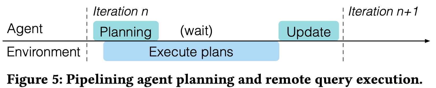
3. Pipelining
   • Parallelize tree search (planning) and remote query execution
   • As soon as main agent thread completes training query planning:
     • Send output plan for remote execution
     • Start planning next query
   • Perform value network update after all plans complete

Value Network

Architecture

• Use Tree Convolution Networks (0.7M parameters, 2.9MB)
• Also experimented with Transformer but similar effect with higher computational cost

Input Encoding

1. Plan encoding: Use same method as Neo
2. Query encoding: simpler ``` [table → selectivity] vector
   • Each slot corresponds to table
   • Store estimated selectivity values
   • Fill absent table slots with 0 ```

Training Process

• Data split:
  • 90% of experience data ($D_{real}$ or $D_{sim}$) → training
  • 10% of experience data → validation (early stopping)
• Loss function:
  • Use L2 loss
  • Predicted latency vs actual latency
• Optimization:
  • Update parameters with SGD
  • Early stopping if validation set performance doesn’t improve
• Label correction:
  • Model output $V_{real}(q,p)$ updated not with actual latency $l$ but
  • With best latency obtained so far for query $q$ containing subplan $p$

---

6. Experiments

Experimental Setup

Workloads:

• Join Order Benchmark (JOB): 113 analytical queries, 3-16 joins (average 8)
  • Random Split: Random split (94 training, 19 test)
  • Slow Split: 19 slowest queries as test set
• TPC-H: Standard analytical benchmark (70 training, 10 test)

Comparison Targets:

• PostgreSQL 12.5 (open source)
• CommDB (commercial DBMS, anonymized)

Environment: Azure VM (8 cores, 64GB RAM, SSD), NVIDIA Tesla M60 GPU

---

Balsa Performance

Overall Performance:

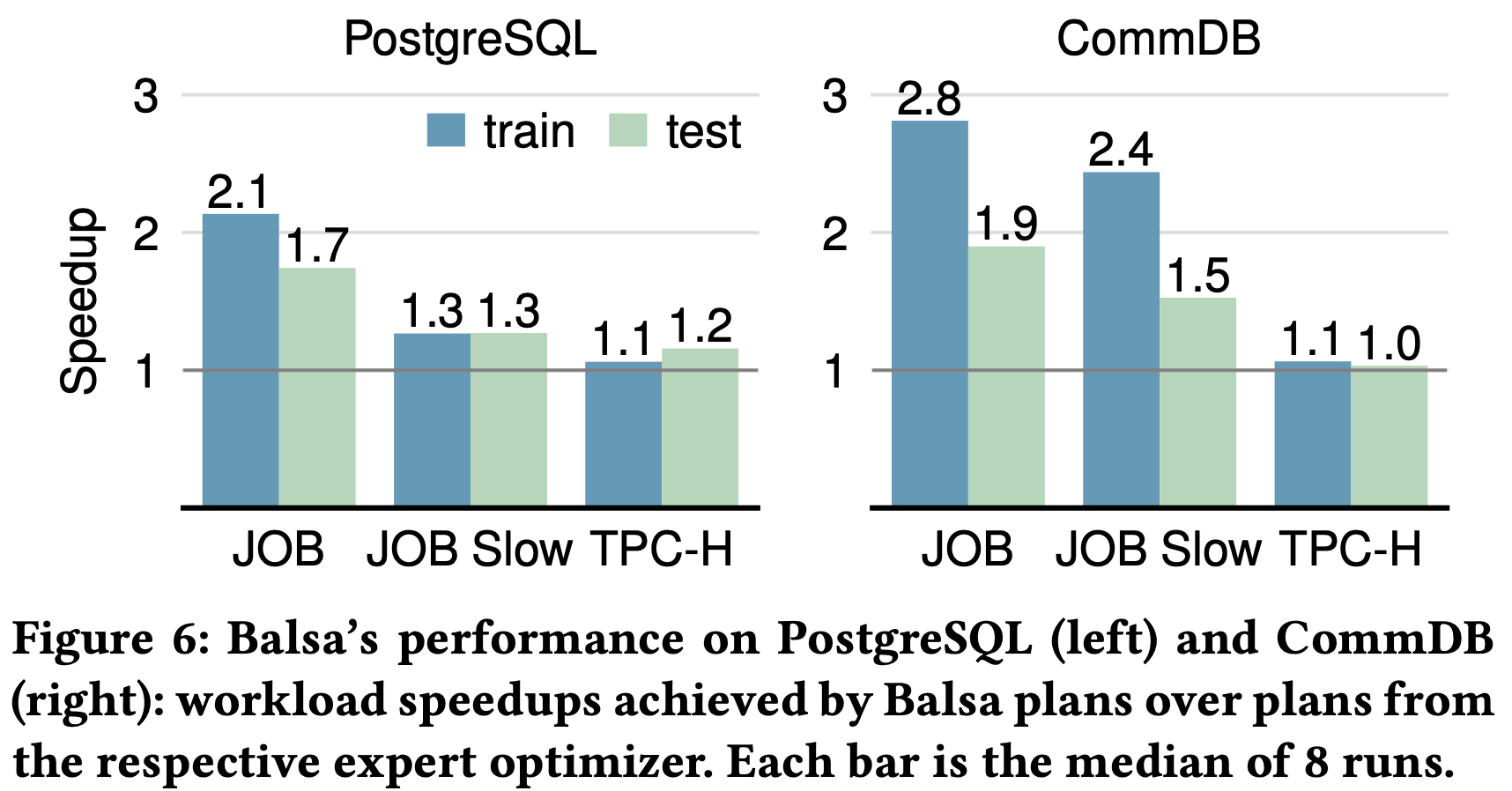
• vs PostgreSQL: 1.1-2.1× speedup on training set, 1.2-1.7× on test set
• vs CommDB: 1.1-2.8× speedup on training set, 1.0-1.9× on test set

Learning Efficiency:

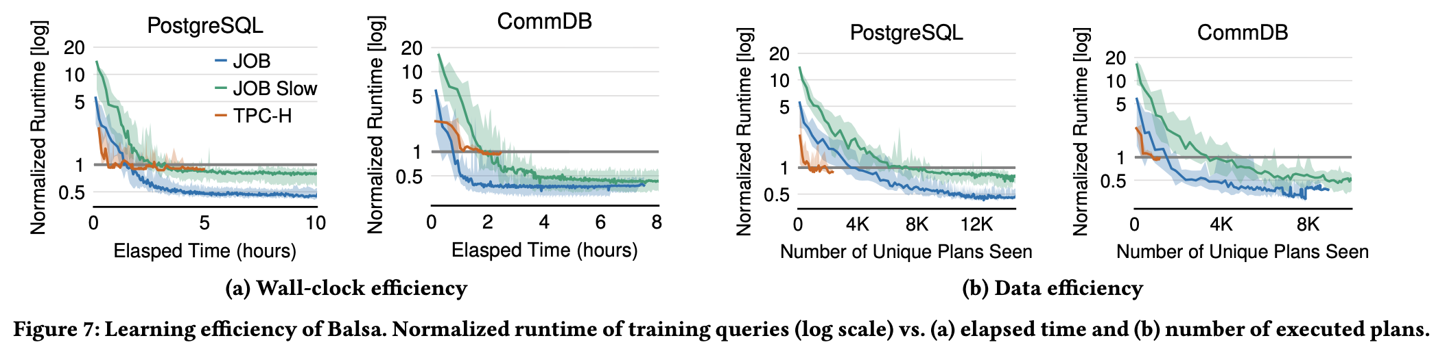
• Time Efficiency: Achieve expert performance within 1-3 hours, peak performance after 4-5 hours
• Data Efficiency: Reach expert performance with thousands of executions

---

Design Choice Analysis

Impact of Initial Simulator:

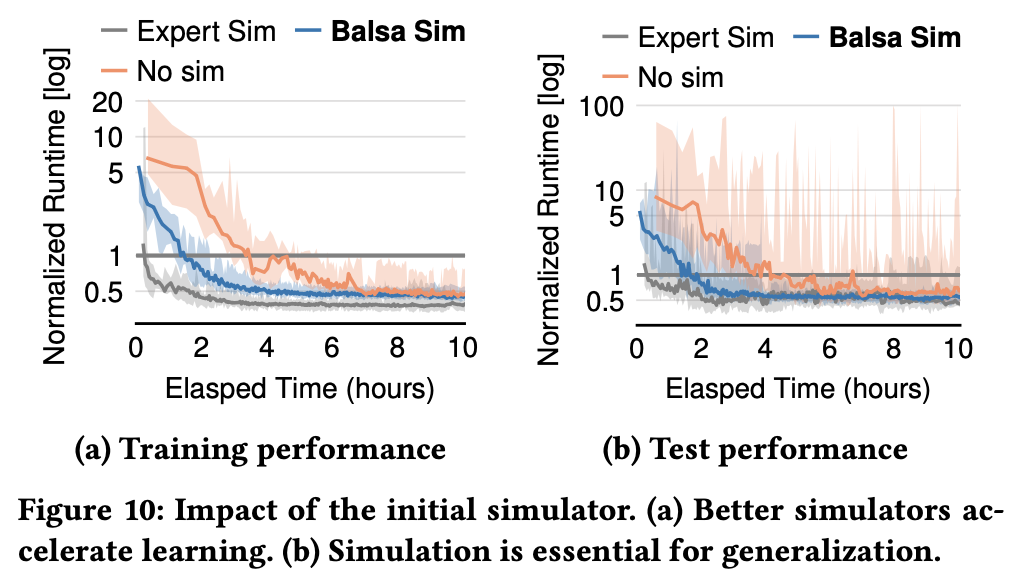
• Unstable generalization performance without simulation
• Expert simulator > Balsa simulator > No simulation

Timeout Mechanism:

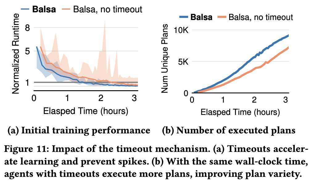
• 35% faster learning, prevents unpredictable performance degradation

Exploration Strategy:

• count-based exploration: chooses the best unseen plan from beam search outputs
• $\epsilon$-greedy beam search: at each step of the search, with a small probability ϵ the beam is “collapsed” into one state

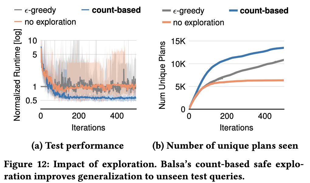
• Count-based safe exploration superior to ε-greedy generalization

Training Method:

• on-policy: uses the latest iteration’s data to update Vreal
• retrain: re-initialize Vreal and retrain on the entire experience(Dreal) at every iteration. Last iteration’s Vreal is discarded.

• On-policy learning 2.1× faster than retraining method

Planning Time Impact:

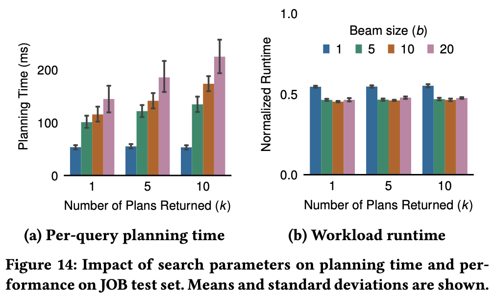
• Average planning time under 250ms in all settings
• Slight performance degradation at beam size b=1 (=greedy search), others similar
• Can reduce planning time 2× at deployment with b=5, k=1 (no performance loss)

---

Comparison with Expert Demonstration Learning

vs Neo:

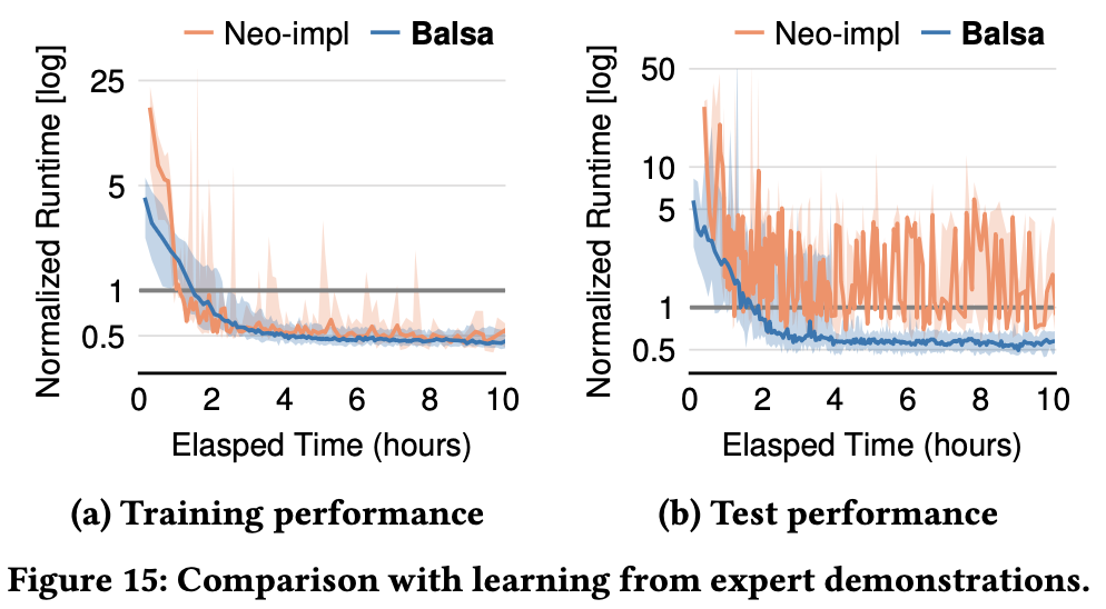
• Balsa 5× faster initial performance
• Neo has high variance and unstable generalization
• Balsa much more efficient: 25 hours vs 2.6 hours

vs Bao:

Balsa vs. Bao: speedups with respect to PostgreSQL

	JOB, train	JOB, test	JOB Slow, train	JOB Slow, test
Balsa	2.1×	1.7×	1.3×	1.3×
Bao	1.6×	1.8×	1.2×	1.1×

• Balsa equal or superior in most cases

---

Generalization Performance Improvement

Diversified Experiences:
Method:

• Merge experiences from 8 independently trained agents
• Retrain new agent with merged experience (no execution)

Effect: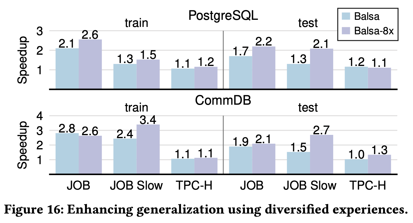

• PostgreSQL: Improvement from 1.7× → 2.2× on JOB test
• CommDB: Significant improvement from 1.5× → 3.4× on JOB Slow test
• Training performance also improves simultaneously

---

Analysis of Learned Behavior

Operator Preference Changes:

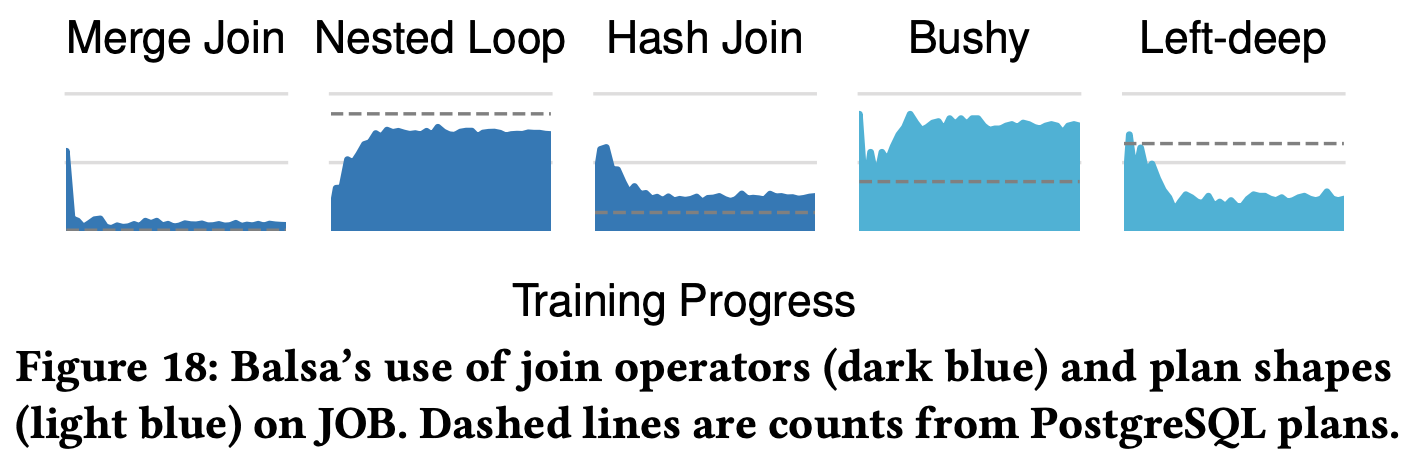
• Merge join: Usage decreases to under 10% after 25 iterations
• Nested loop join: 85% preferred as efficient indexed variant
• Hash join: Maintained at appropriate level for environment

Plan Shapes:

• Shows distinct differences from experts
• Learns preferences specialized for workload and hardware
• Expert is general-purpose, Balsa is specialized optimization

Learning Process:

• Early: Quickly avoid operators/shapes causing high runtime
• Later: Prefer choices efficient in current environment
• New preferences customized for given workload and hardware